(点击
上方蓝字
,快速关注我们)
编译:伯乐在线 - Ree Ray
如有好文章投稿,请点击 → 这里了解详情
情感分析(Sentiment analysis)是自然语言处理(NLP)方法中常见的应用,尤其是以提炼文本情绪内容为目的的分类。利用情感分析这样的方法,可以通过情感评分对定性数据进行定量分析。虽然情感充满了主观性,但情感定量分析已经有许多实用功能,例如企业藉此了解用户对产品的反映,或者判别在线评论中的仇恨言论。
情感分析最简单的形式就是借助包含积极和消极词的字典。每个词在情感上都有分值,通常 +1 代表积极情绪,-1 代表消极。接着,我们简单累加句子中所有词的情感分值来计算最终的总分。显而易见,这样的做法存在许多缺陷,最重要的就是忽略了语境(context)和邻近的词。例如一个简单的短语“not good”最终的情感得分是 0,因为“not”是 -1,“good”是 +1。正常人会将这个短语归类为消极情绪,尽管有“good”的出现。
另一个常见的做法是以文本进行“词袋(bag of words)”建模。我们把每个文本视为 1 到 N 的向量,N 是所有词汇(vocabulary)的大小。每一列是一个词,对应的值是这个词出现的次数。比如说短语“bag of bag of words”可以编码为 [2, 2, 1]。这个值可以作为诸如逻辑回归(logistic regression)、支持向量机(SVM)的机器学习算法的输入,以此来进行分类。这样可以对未知的(unseen)数据进行情感预测。注意这需要已知情感的数据通过监督式学习的方式(supervised fashion)来训练。虽然和前一个方法相比有了明显的进步,但依然忽略了语境,而且数据的大小会随着词汇的大小增加。
Word2Vec 和 Doc2Vec
近几年,Google 开发了名为 Word2Vec 新方法,既能获取词的语境,同时又减少了数据大小。Word2Vec 实际上有两种不一样的方法:CBOW(Continuous Bag of Words,连续词袋)和 Skip-gram。对于 CBOW,目标是在给定邻近词的情况下预测单独的单词。Skip-gram 则相反:我们希望给定一个单独的词(见图 1)来预测某个范围的词。两个方法都使用人工神经网络(Artificial Neural Networks)来作为它们的分类算法。首先,词汇表中的每个单词都是随机的 N 维向量。在训练过程中,算法会利用 CBOW 或者 Skip-gram 来学习每个词的最优向量。
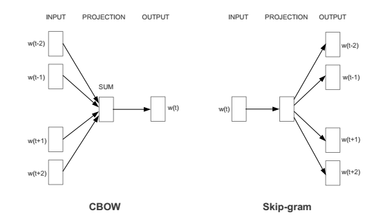
图 1:CBOW 以及 Skip-Gram 结构图,选自《Efficient Estimation of Word Representations in Vector Space》。W(t) 代表当前的单词,而w(t-2), w(t-1) 等则是邻近的单词。
这些词向量现在可以考虑到上下文的语境了。这可以看作是利用基本的代数式来挖掘词的关系(例如:“king” – “man” + “woman” = “queen”)。这些词向量可以作为分类算法的输入来预测情感,有别于词袋模型的方法。这样的优势在于我们可以联系词的语境,并且我们的特征空间(feature space)的维度非常低(通常约为 300,相对于约为 100000 的词汇)。在神经网络提取出这些特征之后,我们还必须手动创建一小部分特征。由于文本长度不一,将以全体词向量的均值作为分类算法的输入来归类整个文档。
然而,即使使用了上述对词向量取均值的方法,我们仍然忽略了词序。Quoc Le 和 Tomas Mikolov 提出了 Doc2Vec 的方法对长度不一的文本进行描述。这个方法除了在原有基础上添加 paragraph / document 向量以外,基本和 Word2Vec 一致,也存在两种方法:DM(Distributed Memory,分布式内存)和分布式词袋(DBOW)。DM 试图在给定前面部分的词和 paragraph 向量来预测后面单独的单词。即使文本中的语境在变化,但 paragraph 向量不会变化,并且能保存词序信息。DBOW 则利用paragraph 来预测段落中一组随机的词(见图 2)。

图 2: Doc2Vec 方法结构图,选自《Distributed Representations of Sentences and Documents》。
一旦经过训练,paragraph 向量就可以作为情感分类器的输入而不需要所有单词。这是目前对 IMDB 电影评论数据集进行情感分类最先进的方法,错误率只有 7.42%。当然,如果这个方法不实用,说这些都没有意义。幸运的是,一个 Python 第三方库 gensim 提供了 Word2Vec 和 Doc2Vec 的优化版本。
基于 Python 的 Word2Vec 举例
在本节我们将会展示怎么在情感分类任务中使用词向量。gensim 这个库是 Anaconda 发行版中的标配,你同样可以利用 pip 来安装。利用它你可以在自己的语料库(一个文档数据集)中训练词向量或者导入 C text 或二进制格式的已经训练好的向量。
from
gensim
.
models
.
word2vec
import
Word2Vec
model
=
Word2Vec
.
load_word2vec_format
(
'vectors.txt'
,
binary
=
False
)
#C text 格式
model
=
Word2Vec
.
load_word2vec_format
(
'vectors.bin'
,
binary
=
True
)
#二进制格式
我发现读取谷歌已经训练好的词向量尤其管用,这些向量来自谷歌新闻(Google News),由超过千亿级别的词训练而成,“已经训练过的词和短语向量”可以在这里找到。注意未压缩的文件有 3.5 G。通过 Google 词向量我们能够发现词与词之间有趣的关联:
from
gensim
.
models
.
word2vec
import
Word2Vec
model
=
Word2Vec
.
load_word2vec_format
(
'GoogleNews-vectors-negative300.bin'
,
binary
=
True
)
model
.
most_similar
(
positive
=
[
'woman'
,
'king'
],
negative
=
[
'man'
],
topn
=
5
)
[(
u
'queen'
,
0.711819589138031
),
(
u
'monarch'
,
0.618967592716217
),
(
u
'princess'
,
0.5902432799339294
),
(
u
'crown_prince'
,
0.5499461889266968
),
(
u
'prince'
,
0.5377323031425476
)]
有趣的是它可以发现语法关系,例如识别最高级(superlatives)和动词词干(stems):
“biggest” – “big” + “small” = “smallest”
model
.
most_similar
(
positive
=
[
'biggest'
,
'small'
],
negative
=
[
'big'
],
topn
=
5
)
[(
u
'smallest'
,
0.6086569428443909
),
(
u
'largest'
,
0.6007465720176697
),
(
u
'tiny'
,
0.5387299656867981
),
(
u
'large'
,
0.456944078207016
),
(
u
'minuscule'
,
0.43401968479156494
)]
“ate” – “eat” + “speak” = “spoke”
model
.
most_similar
(
positive
=
[
'ate'
,
'speak'
],
negative
=
[
'eat'
],
topn
=
5
)
[(
u
'spoke'
,
0.6965223550796509
),
(
u
'speaking'
,
0.6261293292045593
),
(
u
'conversed'
,
0.5754593014717102
),
(
u
'spoken'
,
0.570488452911377
),
(
u
'speaks'
,
0.5630602240562439
)]
由以上例子可以清楚认识到 Word2Vec 能够学习词与词之间的有意义的关系。这也就是为什么它对于许多 NLP 任务有如此大的威力,包括在本文中的情感分析。在我们用它解决起情感分析问题以前,让我们先测试一下 Word2Vec 对词分类(separate)和聚类(cluster)的本事。我们会用到三个示例词集:食物类(food)、运动类(sports)和天气类(weather),选自一个非常棒的网站 Enchanted Learning。因为这些向量有 300 个维度,为了在 2D 平面上可视化,我们会用到 Scikit-Learn’s 中叫作“t-SNE”的降维算法操作
首先必须像下面这样取得词向量:
import
numpy
as
np
with
open
(
'food_words.txt'
,
'r'
)
as
infile
:
food_words
=
infile
.
readlines
()
with
open
(
'sports_words.txt'
,
'r'
)
as
infile
:
sports_words
=
infile
.
readlines
()
with
open
(
'weather_words.txt'
,
'r'
)
as
infile
:
weather_words
=
infile
.
readlines
()
def
getWordVecs
(
words
)
:
vecs
=
[]
for
word
in
words
:
word
=
word
.
replace
(
'n'
,
''
)
try
:
vecs
.
append
(
model
[
word
].
reshape
((
1
,
300
)))
except
KeyError
:
continue
vecs
=
np
.
concatenate
(
vecs
)
return
np
.
array
(
vecs
,
dtype
=
'float'
)
#TSNE expects float type values
food_vecs
=
getWordVecs
(
food_words
)
sports_vecs
=
getWordVecs
(
sports_words
)
weather_vecs
=
getWordVecs
(
weather_words
)
我们接着使用 TSNE 和 matplotlib 可视化聚类,代码如下:
from
sklearn
.
manifold
import
TSNE
import
matplotlib
.
pyplot
as
plt
ts
=
TSNE
(
2
)
reduced_vecs
=
ts
.
fit_transform
(
np
.
concatenate
((
food_vecs
,
sports_vecs
,
weather_vecs
)))
#color points by word group to see if Word2Vec can separate them
for
i
in
range
(
len
(
reduced_vecs
))
:
if
i
&
lt
;
len
(
food_vecs
)
:
#food words colored blue
color
=
'b'
elif
i
&
gt
;
=
len
(
food_vecs
)
and
i
&
lt
;
(
len
(
food_vecs
)
+
len
(
sports_vecs
))
:
#sports words colored red
color
=
'r'
else
:
#weather words colored green
color
=
'g'
plt
.
plot
(
reduced_vecs
[
i
,
0
],
reduced_vecs
[
i
,
1
],
marker
=
'o'
,
color
=
color
,
markersize
=
8
)
import
numpy
as
np
with
open
(
'food_words.txt'
,
'r'
)
as
infile
:
food_words
=
infile
.
readlines
()
with
open
(
'sports_words.txt'
,
'r'
)
as
infile
:
sports_words
=
infile
.
readlines
()
with
open
(
'weather_words.txt'
,
'r'
)
as
infile
:
weather_words
=
infile
.
readlines
()
def
getWordVecs
(
words
)
:
vecs
=
[]
for
word
in
words
:
word
=
word
.
replace
(
'n'
,
''
)
try
:
vecs
.
append
(
model
[
word
].
reshape
((
1
,
300
)))
except
KeyError
:
continue
vecs
=
np
.
concatenate
(
vecs
)
return
np
.
array
(
vecs
,
dtype
=
'float'
)
#TSNE 要求浮点型的值
food_vecs
=
getWordVecs
(
food_words
)
sports_vecs
=
getWordVecs
(
sports_words
)
weather_vecs
=
getWordVecs
(
weather_words
)
结果如下:
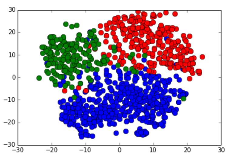
图 3:食物类单词(蓝色),运动类单词(红色)和天气类单词(绿色)T-SNE 集群效果图。
我们可以从上面的例子看到,Word2Vec 不仅能有效分类不相关的单词,同样也能聚类类似的词。
推特 Emoji 情感分析
现在我们进入下一个例程,利用符号表情作为搜索词的推特情感分析。我们把这些符号表情作为我们数据的“模糊(fuzzy)”标签;微笑表情(:-))与积极情绪对应,而皱眉表情(:-()则对应消极情绪。在大约 400,000 条推特数据中,积极和消极的各占一半(even split)。我们对积极和消极情绪的推特进行了随机采样,并按80 / 20 的比例分为了训练集/ 测试集。我们接着在 Word2Vec 模型上训练推特。为了避免数据泄露(data leakage),在训练数据集分类完成以前我们都不会在 Word2Vec 上训练。为了结构化分类器的输入,我们对所有推特词向量取均值。我们会用到 Scikit-Learn 这个第三方库做大量的机器学习。
我们首先导入我们的数据并训练 Word2Vec 模型
from
sklearn
.
cross_validation
import
train_test_split
from
gensim
.
models
.
word2vec
import
Word2Vec
with
open
(
'twitter_data/pos_tweets.txt'
,
'r'
)
as
infile
:
pos_tweets
=
infile
.
readlines
()
with
open
(
'twitter_data/neg_tweets.txt'
,
'r'
)
as
infile
:
neg_tweets
=
infile
.
readlines
()
# 1 代表积极情绪,0 代表消极情绪
y
=
np
.
concatenate
((
np
.
ones
(
len
(
pos_tweets
)),
np
.
zeros
(
len
(
neg_tweets
))))
x_train
,
x_test
,
y_train
,
y_test
=
train_test_split
(
np
.
concatenate
((
pos_tweets
,
neg_tweets
)),
y
,
test_size
=
0.2
)
# 零星的预处理
def
cleanText
(
corpus
)
:
corpus
=
[
z
.
lower
().
replace
(
'n'
,
''
).
split
()
for
z
in
corpus
]
return
corpus
x_train
=
cleanText
(
x_train
)
x_test
=
cleanText
(
x_test
)
n_dim
=
300
# 初始化模型并创建词汇表(vocab)
imdb_w2v
=
Word2Vec
(
size
=
n_dim
,
min_count
=
10
)
imdb_w2v
.
build_vocab
(
x_train
)
# 训练模型 (会花费几分钟)
imdb_w2v
.
train
(
x_train
)
下面我们必须对输入文本创建词向量,为了平均推特中的所有词向量,将用到如下的函数:
# 对训练数据集创建词向量,接着进行比例缩放(scale)。
def
buildWordVector
(
text
,
size
)
:
vec
=
np
.
zeros
(
size
).
reshape
((
1
,
size
))
count
=
0.
for
word
in
text
:
try
:
vec
+=
imdb_w2v
[
word
].
reshape
((
1
,
size
))
count
+=
1.
except
KeyError
:
continue
if
count
!=
0
:
vec
/=
count
return
vec
对我们的数据集进行缩放是标准化处理的一部分。通过均值为零的高斯分布,意味着大于均值则为积极,小于则为消极。许多机器学习模型要求使用缩放过的数据集来获得更好的处理效果,尤其是多特征(例如文本分类)。
from
sklearn
.
preprocessing
import
scale
train_vecs
=
np
.
concatenate
([
buildWordVector
(
z
,
n_dim
)
for
z
in
x_train
])
train_vecs
=
scale
(
train_vecs
)
# 在测试推特数据集中训练 Word2Vec
imdb_w2v
.
train
(
x_test
)
最终我们必须创建测试数据向量并进行比例缩放来评估。
# 创建测试推特向量并缩放
test_vecs
=
np
.
concatenate
([
buildWordVector
(
z
,
n_dim
)
for
z
in
x_test
])
test_vecs
=
scale
(
test_vecs
)
下面我们想通过计算测试数据的预测精度来验证我们的分类器,同时测试它们的 ROC 曲线(Receiver Operating Characteristic,受试者操作特征曲线)。当模型参数调节时,ROC 曲线会测试分类器的真阳性(true-positive)以及假阳性(false-positive)。本例中,我们通过调节边界阈值概率(cut-off threshold probability)将某条推特分类为积极或消极情绪。通常,更希望得到最大化的真阳性和最小化的假阳性,也就是 ROC 曲线下方最大的区域(AUC)。通过这里更多地了解 ROC 曲线。
开始训练我们的分类器,本例对逻辑回归(Logistic Regression)使用随机梯度下降(Stochastic Gradient Descent)。
# 使用分类算法(例如:随机逻辑回归(Stochastic Logistic Regression)来训练数据集,接着从 sklearn.linear_model 导入 SGDClassifier 进行模型处理)
lr
=
SGDClassifier
(
loss
=
'log'
,
penalty
=
'l1'
)
lr
.
fit
(
train_vecs
,
y_train
)
print
'Test Accuracy: %.2f'
%
lr
.
score
(
test_vecs
,
y_test
)
我们利用 matplotlib 和 Scikit-Learn 的 metric 包中的 roc_curve 创建 ROC 曲线来评估。
# 创建 ROC 曲线
from
sklearn
.
metrics


