(点击
上方公众号
,可快速关注)
来源:hainingwyx
链接:www.jianshu.com/p/59b510bafb4d
写
在之前
想看程序参数说明的请到:
-
http://scikit-learn.org/stable/modules/generated/sklearn.tree.DecisionTreeClassifier.html
-
http://scikit-learn.org/stable/modules/generated/sklearn.tree.DecisionTreeRegressor.html#sklearn.tree.DecisionTreeRegressor
-
http://www.th7.cn/Program/Python/201604/830424.shtml
本文是Scikit-learn中的决策树算法的原理、应用的介绍。
正文部分
决策树是一个非参数的监督式学习方法,主要用于分类和回归。算法的目标是通过推断数据特征,学习决策规则从而创建一个预测目标变量的模型。如下如所示,决策树通过一系列if-then-else 决策规则 近似估计一个正弦曲线。
决策树优势:
-
简单易懂,原理清晰,决策树可以实现可视化
-
数据准备简单。其他的方法需要实现数据归一化,创建虚拟变量,删除空白变量。(注意:这个模块不支持缺失值)
-
使用决策树的代价是数据点的对数级别。
-
能够处理数值和分类数据
-
能够处理多路输出问题
-
使用白盒子模型(内部结构可以直接观测的模型)。一个给定的情况是可以观测的,那么就可以用布尔逻辑解释这个结果。相反,如果在一个黑盒模型(ANN),结果可能很难解释
-
可以通过统计学检验验证模型。这也使得模型的可靠性计算变得可能
-
即使模型假设违反产生数据的真实模型,表现性能依旧很好。
决策树劣势:
-
可能会建立过于复杂的规则,即过拟合。为避免这个问题,剪枝、设置叶节点的最小样本数量、设置决策树的最大深度有时候是必要的。
-
决策树有时候是不稳定的,因为数据微小的变动,可能生成完全不同的决策树。 可以通过总体平均(ensemble)减缓这个问题。应该指的是多次实验。
-
学习最优决策树是一个NP完全问题。所以,实际决策树学习算法是基于试探性算法,例如在每个节点实现局部最优值的贪心算法。这样的算法是无法保证返回一个全局最优的决策树。可以通过随机选择特征和样本训练多个决策树来缓解这个问题。
-
有些问题学习起来非常难,因为决策树很难表达。如:异或问题、奇偶校验或多路复用器问题
-
如果有些因素占据支配地位,决策树是有偏的。因此建议在拟合决策树之前先平衡数据的影响因子。
分类
DecisionTreeClassifier 能够实现多类别的分类。输入两个向量:向量X,大小为[n_samples,n_features],用于记录训练样本;向量Y,大小为[n_samples],用于存储训练样本的类标签。
from sklearn import
tree
X
=
[[
0
,
0
],
[
1
,
1
]]
Y
=
[
0
,
1
]
clf
=
tree
.
DecisionTreeClassifier
()
clf
=
clf
.
fit
(
X
,
Y
)
clf
.
predict
([[
2.
,
2.
]])
clf
.
predict_proba
([[
2.
,
2.
]])
#计算属于每个类的概率
能够实现二进制分类和多分类。使用Isis数据集,有:
from
sklearn
.
datasets import load_iris
from sklearn import tree
iris
=
load_iris
()
clf
=
tree
.
DecisionTreeClassifier
()
clf
=
clf
.
fit
(
iris
.
data
,
iris
.
target
)
# export the tree in Graphviz format using the export_graphviz exporter
with open
(
"iris.dot"
,
'w'
)
as
f
:
f
=
tree
.
export_graphviz
(
clf
,
out_file
=
f
)
# predict the class of samples
clf
.
predict
(
iris
.
data
[
:
1
,
:
])
# the probability of each class
clf
.
predict_proba
(
iris
.
data
[
:
1
,
:
])
安装Graphviz将其添加到环境变量,使用dot创建一个PDF文件。dot -Tpdf iris.dot -o iris.pdf
# 删除dot文件
import os
os
.
unlink
(
'iris.dot'
)
如果安装了pydotplus,也可以在Python中直接生成:
import pydotplus
dot_data
=
tree
.
export_graphviz
(
clf
,
out_file
=
None
)
graph
=
pydotplus
.
graph_from_dot_data
(
dot_data
)
graph
.
write_pdf
(
"iris.pdf"
)
可以根据不同的类别输出不同的颜色,也可以指定类别名字。
from
IPython
.
display import Image
dot_data
=
tree
.
export_graphviz
(
clf
,
out_file
=
None
,
feature_names
=
iris
.
feature_names
,
class_names
=
iris
.
target_names
,
filled
=
True
,
rounded
=
True
,
special_characters
=
True
)
graph
=
pydotplus
.
graph_from_dot_data
(
dot_data
)
Image
(
graph
.
create_png
())
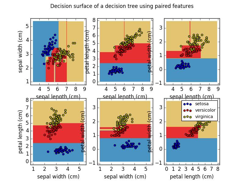
更多地可以看到分类的效果:
回归
和分类不同的是向量y可以是浮点数。
from sklearn import
tree
X
=
[[
0
,
0
],
[
2
,
2
]]
y
=
[
0.5
,
2.5
]
clf
=
tree
.
DecisionTreeRegressor
()
clf
=
clf
.
fit
(
X
,
y
)
clf
.
predict
([[
1
,
1
]])
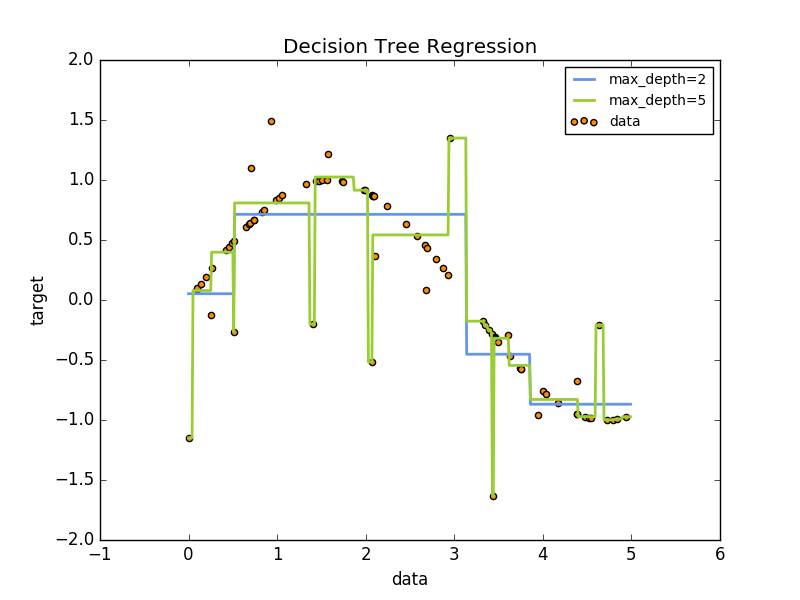
本文前面提到的例子:http://scikit-learn.org/stable/auto_examples/tree/plot_tree_regression.html#sphx-glr-auto-examples-tree-plot-tree-regression-py
# Import the necessary modules and libraries
import numpy
as
np
from
sklearn
.
tree import DecisionTreeRegressor
import
matplotlib
.
pyplot
as
plt
# Create a random dataset
rng
=
np
.
random
.
RandomState
(
1
)
X
=
np
.
sort
(
5
*
rng
.
rand
(
80
,
1
),
axis
=
0
)
y
=
np
.
sin
(
X
).
ravel
()
y
[
::
5
]
+=
3
*
(
0.5
-
rng
.
rand
(
16
))
# Fit regression model
regr_1
=
DecisionTreeRegressor
(
max_depth
=
2
)
regr_2
=
DecisionTreeRegressor
(
max_depth
=
5
)
regr_1
.
fit
(
X
,
y
)
regr_2
.
fit
(
X
,
y
)
# Predict
X_test
=
np
.
arange
(
0.0
,
5.0
,
0.01
)[
:
,
np
.
newaxis
]
y_1
=
regr_1
.
predict
(
X_test
)
y_2
=
regr_2
.
predict
(
X_test
)
# Plot the results
plt
.
figure
()
plt
.
scatter
(
X
,
y
,
c