
简介
在本教程中,我们将对来自10X和snATAC-seq技术产生的成年小鼠大脑的单细胞ATAC-seq测序数据进行整合分析。该示例的所有数据可以从以下链接进行下载:http://renlab.sdsc.edu/r3fang/share/github/Mouse_Brain_10X_snATAC/
分析流程
-
Step 0. Download data
-
Step 1. Create snap object
-
Step 2. Select barcode
-
Step 3. Add cell-by-bin matrix
-
Step 4. Combine snap objects
-
Step 5. Filter bins
-
Step 6. Dimensionality reduction
-
Step 7. Determine significant components
-
Step 8. Remove batch effect
-
Step 9. Graph-based cluster
-
Step 10. Visualization
Step 0. Download data
       # 下载所需的数据集


      $ wget http:

       //renlab.sdsc.edu/r3fang/share/github/Mouse_Brain_10X_snATAC/CEMBA180305_2B.snap


      $ wget http:

       //renlab.sdsc.edu/r3fang/share/github/Mouse_Brain_10X_snATAC/CEMBA180305_2B.barcode.txt


      $ wget http:

       //renlab.sdsc.edu/r3fang/share/github/Mouse_Brain_10X_snATAC/atac_v1_adult_brain_fresh_5k.snap


      $ wget http:

       //renlab.sdsc.edu/r3fang/share/github/Mouse_Brain_10X_snATAC/atac_v1_adult_brain_fresh_5k.barcode.txt
Step 1. Create snap object
首先,我们将所用的两个数据集读取到snap对象列表中。
       #


       加载SnapATAC包


       >


       library(SnapATAC);


       >


       file.list = c(

        "CEMBA180305_2B.snap"

       ,

        "atac_v1_adult_brain_fresh_5k.snap"

       );


       >


       sample.list = c(

        "snATAC"

       ,

        "10X"

       );


       #


       读取snap文件


       >


       x.sp.ls = lapply(seq(file.list),

        function

       (i){


      x.sp = createSnap(file=file.list[i], sample=sample.list[i]);


      x.sp


      })


       >


       names(x.sp.ls) = sample.list;


       #


       查看snap文件信息


       >


       x.sp.ls


       #


        # $snATAC


       #


        # number of barcodes: 15136


       #


        # number of bins: 0


       #


        # number of genes: 0


       #


        # number of peaks: 0


       #


        # number of motifs: 0


       #


        #


       #


        # $`10X`


       #


        # number of barcodes: 20000


       #


        # number of bins: 0


       #


        # number of genes: 0


       #


        # number of peaks: 0


       #


        # number of motifs: 0
Step 2. Select barcode
接下来,我们将读取这两个数据集的barcode信息,并选择高质量的barcodes。
       >


       barcode.file.list = c(

        "CEMBA180305_2B.barcode.txt"

       ,

        "atac_v1_adult_brain_fresh_5k.barcode.txt"

       );


       #


       读取barcode信息


       >


       barcode.list = lapply(barcode.file.list,

        function

       (file){


      read.table(file)[,1];


      })


       >


       x.sp.list = lapply(seq(x.sp.ls),

        function

       (i){


      x.sp = x.sp.ls[[i]];


      x.sp  = x.sp[x.sp@barcode %in% barcode.list[[i]],];


      })


       >


       names(x.sp.list) = sample.list;


       >


       x.sp.list


       #


        # $snATAC


       #


        # number of barcodes: 9646


       #


        # number of bins: 0


       #


        # number of genes: 0


       #


        # number of peaks: 0


       #


        # number of motifs: 0


       #


        #


       #


        # $`10X`


       #


        # number of barcodes: 4100


       #


        # number of bins: 0


       #


        # number of genes: 0


       #


        # number of peaks: 0


       #


        # number of motifs: 0
Step 3. Add cell-by-bin matrix
#
使用addBmatToSnap函数计算cell-by-bin计数矩阵并添加到snap对象中
>
x.sp.list = lapply(seq(x.sp.list),
function
(i){
x.sp = addBmatToSnap(x.sp.list[[i]], bin.size=5000);
x.sp
})
>
x.sp.list
#
# $snATAC
#
# number of barcodes: 9646
#
# number of bins: 545118
#
# number of genes: 0
#
# number of peaks: 0
#
# number of motifs: 0
#
#
#
# $`10X`
#
# number of barcodes: 4100
#
# number of bins: 546206
#
# number of genes: 0
#
# number of peaks: 0
#
# number of motifs: 0
可以看到,这两个snap对象中含有不同数目的bins,这是因为这两个数据集使用的参考基因组有细微的差异。
Step 4. Combine snap objects
接下来,我们将这个数据集进行合并。
To combine these two snap objects, common bins are selected.
       #


       选择两个数据集共有的bins


       >


       bin.shared = Reduce(intersect, lapply(x.sp.list,

        function

       (x.sp) x.sp@feature

        $name

       ));


       >


       x.sp.list function

      (x.sp){


      idy = match(bin.shared, x.sp@feature$name);


      x.sp[,idy, mat="bmat"];


      })


       #


       合并两个数据集


       >


       x.sp = Reduce(snapRbind, x.sp.list);


       >


       rm(x.sp.list);

        # free memory


       >


       gc();


       >


       table(x.sp@sample);


       #


        #   10X snATAC


       #


        #  4100   9646
Step 5. Binarize matrix
       #


       使用makeBinary函数将计数矩阵转换为二进制矩阵


       >


       x.sp = makeBinary(x.sp, mat=

        "bmat"

       );
Step 6. Filter bins
首先,我们将与ENCODE中blacklist区域重叠的bins进行过滤,以防止潜在的artifacts。
       >


       system(

        "wget http://mitra.stanford.edu/kundaje/akundaje/release/blacklists/mm10-mouse/mm10.blacklist.bed.gz"

       );


       >


       library(GenomicRanges);


       >


       black_list = read.table(

        "mm10.blacklist.bed.gz"

       );


       >


       black_list.gr = GRanges(


      black_list[,1],


      IRanges(black_list[,2], black_list[,3])


      );


       >


       idy = queryHits(findOverlaps(x.sp@feature, black_list.gr));


       >


        if

       (length(idy) > 0){x.sp = x.sp[,-idy, mat=

        "bmat"

       ]};


       >


       x.sp


       #


        # number of barcodes: 13746


       #


        # number of bins: 545015


       #


        # number of genes: 0


       #


        # number of peaks: 0


       #


        # number of motifs: 0
接下来,我们将过滤掉那些不需要的染色体信息。
>
chr.exclude = seqlevels(x.sp@feature)[grep(
"random|chrM"
, seqlevels(x.sp@feature))];
>
idy = grep(paste(chr.exclude, collapse=
"|"
), x.sp@feature);
>
if
(length(idy) > 0){x.sp = x.sp[,-idy, mat=
"bmat"
]};
>
x.sp
#
# number of barcodes: 13746
#
# number of bins: 545011
#
# number of genes: 0
#
# number of peaks: 0
#
# number of motifs: 0
第三,bins的覆盖率大致是服从对数正态分布的。我们将与不变特征(如管家基因的启动子)重叠的前5%的bins进行删除 。
       >


       bin.cov = log10(Matrix::colSums(x.sp@bmat)+1);


       >


       bin.cutoff = quantile(bin.cov[bin.cov > 0], 0.95);


       >


       idy =

        which

       (bin.cov <= bin.cutoff="" bin.cov=""> 0);


       >


       x.sp = x.sp[, idy, mat=

        "bmat"

       ];


       >


       x.sp


       #


        # number of barcodes: 13746


       #


        # number of bins: 479127


       #


        # number of genes: 0


       #


        # number of peaks: 0


       #


        # number of motifs: 0
Step 7. Reduce dimensionality
我们使用diffusion maps的方法来计算landmark diffusion maps进行数据降维。首先,我们随机选择出10,000个细胞作为landmarks,然后将剩余的query细胞映射到diffusion maps embedding中。
       >


       row.covs = log10(Matrix::rowSums(x.sp@bmat)+1);


       >


       row.covs.dens = density(


      x = row.covs,


      bw = 'nrd', adjust = 1


      );


       >


       sampling_prob = 1 / (approx(x = row.covs.dens

        $x

       , y = row.covs.dens

        $y

       , xout = row.covs)

        $y

       + .Machine

        $double

       .eps);


       >


       set.seed(1);


       >


       idx.landmark.ds = sort(sample(x = seq(nrow(x.sp)), size = 10000, prob = sampling_prob));


       >


       x.landmark.sp = x.sp[idx.landmark.ds,];


       >


       x.query.sp = x.sp[-idx.landmark.ds,];


       >


       x.landmark.sp = runDiffusionMaps(


      obj= x.landmark.sp,


      input.mat="bmat",


      num.eigs=50


      );


       >


       x.query.sp = runDiffusionMapsExtension(


      obj1=x.landmark.sp,


      obj2=x.query.sp,


      input.mat="bmat"


      );


       >


       x.landmark.sp@metaData

        $landmark

       = 1;


       >


       x.query.sp@metaData

        $landmark

       = 0;


       >


       x.sp = snapRbind(x.landmark.sp, x.query.sp);


       #


        # combine landmarks and query cells;


       >


       x.sp = x.sp[order(x.sp@sample),];

        # IMPORTANT


       >


       rm(x.landmark.sp, x.query.sp);

        # free memory
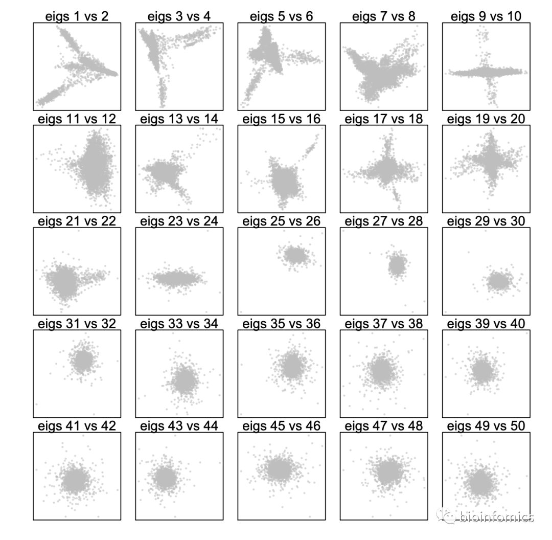
Step 8. Determine significant components
      > plotDimReductPW(


      obj=x.sp,


      eigs.dims=

       1

      :

       50

      ,


      point.size=

       0.3

      ,


      point.color=

       "grey"

      ,


      point.shape=

       19

      ,


      point.alpha=

       0.6

      ,


      down.sample=

       5000

      ,


      pdf.file.name=

       NULL

      ,


      pdf.height=

       7

      ,


      pdf.width=

       7


      );
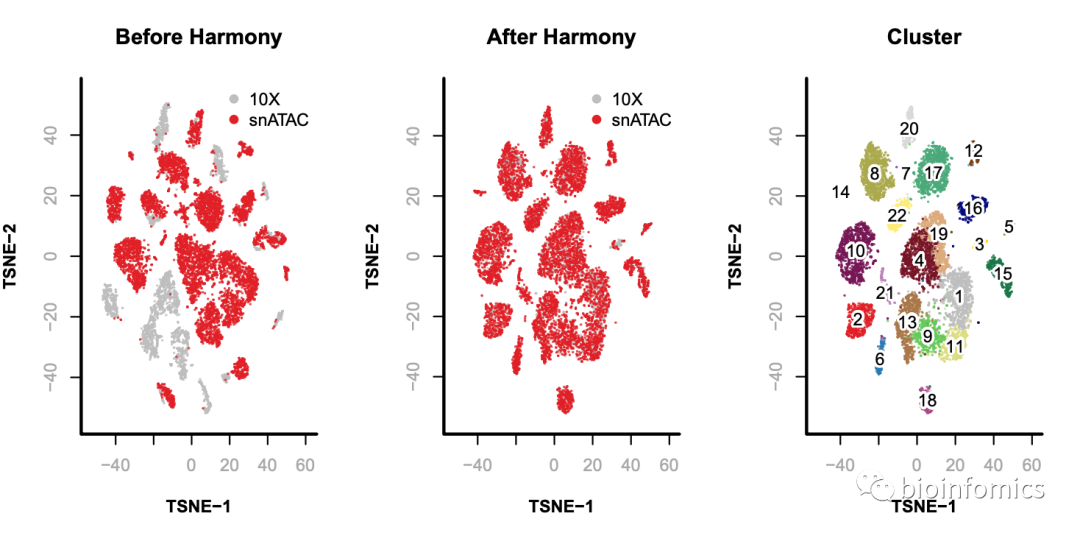
Step 9. Remove batch effect
      > library(harmony);


       # 使用runHarmony函数进行批次校正


      > x.after.sp = runHarmony(


      obj=x.sp,


      eigs.dims=

       1


