基因共表达聚类分析及可视化

新出炉的Cytoscape视频教程 共表达基因的寻找是转录组分析的一个部分，样品多可以使用 WGCNA ，样品少可直接通过聚类分析如 K-means 、 K-medoids (比K-means更稳定)或 Hcluster 或设定 pearson correlation 阈值来选择共表达基因。

下面将实战演示 K-means 、 K-medoids 聚类操作和常见问题：如何聚类分析，如何确定合适的 cluster数目 ，如何绘制 共表达 密度图、线图、热图、网络图等。

获得模拟数据集

MixSim 是用来评估聚类算法效率生成模拟数据集的一个R包。

library(MixSim)
# 获得5个中心点，8维属性的数据模型    
data = MixSim(MaxOmega=0,  K=5,  p=8,  ecc=0.5,  int=c(10, 100))
# 根据模型获得1000次观察的数据集
A 1000,  Pi=data$Pi, Mu=data$Mu, S=data$S, n.out=0)
data # 数据标准化
data 1, scale))
# 定义行列名字
rownames(data) "Gene", 1:1000, sep="_")
colnames(data) 1:8]
head(data)

##                  a          b         c        d         e          f
## Gene_1 -0.04735251 -0.7147304 0.3836436 1.322786 0.9718988 -0.5468517
## Gene_2  0.09276733 -0.8066507 0.5476909 1.351780 0.8679073 -0.6019107
## Gene_3 -0.08751894 -0.6461075 0.4371506 1.522767 0.8031865 -0.6904081
## Gene_4  0.11065988 -0.7327674 0.4550544 1.379773 0.9304277 -0.5532253
## Gene_5 -0.02722127 -0.7833089 0.6700604 1.448916 0.7128284 -0.6266295
## Gene_6  0.15119823 -0.7468292 0.4859932 1.351159 0.9179421 -0.5625206
##                g         h
## Gene_1 0.4127370 -1.782130
## Gene_2 0.2852284 -1.736813
## Gene_3 0.3420581 -1.681128
## Gene_4 0.1808146 -1.770737
## Gene_5 0.2936467 -1.688292
## Gene_6 0.1821925 -1.779136

K-means

K-means 称为K-均值聚类；k-means聚类的基本思想是根据预先设定的分类数目，在样本空间随机选择相应数目的点做为起始聚类中心点；然后将空间中到每个起始中心点距离最近的点作为一个集合，完成第一次聚类；获得第一次聚类集合所有点的平均值做为新的中心点，进行第二次聚类；直到得到的聚类中心点不再变化或达到尝试的上限，则完成了聚类过程。

聚类模拟如下图：

聚类过程需要考虑下面3点：

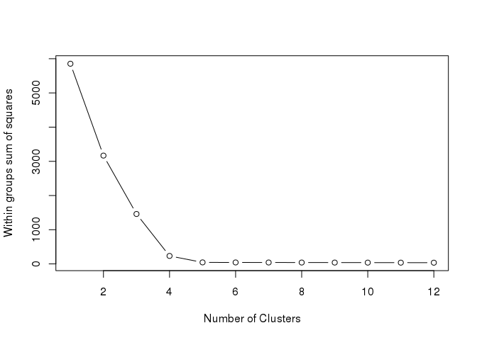
1.需要确定聚出的类的数目。可通过遍历多个不同的聚类数计算其类内平方和的变化，并绘制线图，一般选择类内平方和降低开始趋于平缓的聚类数作为较优聚类数, 又称 elbow算法 。下图中拐点很明显， 5 。

tested_cluster 12
wss 1) * sum(apply(data, 2, var))
for (i in 2:tested_cluster) {
    wss[i] 100,  nstart=25)$tot.withinss
}
plot(1:tested_cluster, wss, type="b", xlab="Number of Clusters", ylab="Within groups sum of squares")

2.K-means聚类起始点为随机选取，容易获得局部最优，需重复计算多次，选择最优结果。

library(cluster)
library(fpc)
# iter.max: 最大迭代次数
# nstart: 选择的随机集的数目
# centers: 上一步推测出的最优类数目
center = 5
fit 100, nstart=25)
withinss print(paste("Get withinss for the first run", withinss))

## [1] "Get withinss for the first run 44.381088289378"

try_count = 10
for (i in 1:try_count) {
  tmpfit 100, nstart=25)
  tmpwithinss   print(paste(("The additional "), i, 'run, withinss', tmpwithinss))
  if (tmpwithinss < withinss){
    withins     fit   }
}

## [1] "The additional  1 run, withinss 44.381088289378"
## [1] "The additional  2 run, withinss 44.381088289378"
## [1] "The additional  3 run, withinss 44.381088289378"
## [1] "The additional  4 run, withinss 44.381088289378"
## [1] "The additional  5 run, withinss 44.381088289378"
## [1] "The additional  6 run, withinss 44.381088289378"
## [1] "The additional  7 run, withinss 44.381088289378"
## [1] "The additional  8 run, withinss 44.381088289378"
## [1] "The additional  9 run, withinss 44.381088289378"
## [1] "The additional  10 run, withinss 44.381088289378"

fit_cluster = fit$cluster

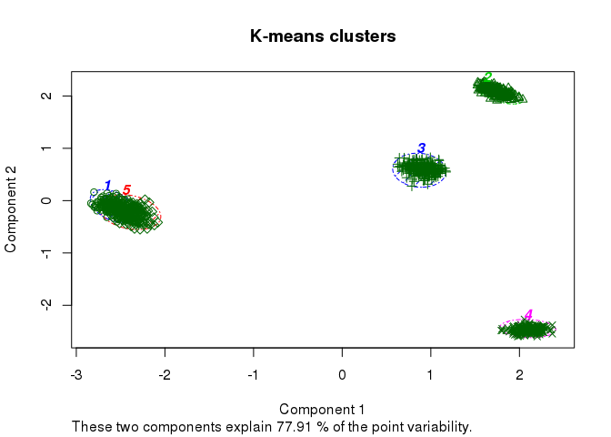
简单绘制下聚类效果

clusplot(data, fit_cluster, shade=T, labels=5, lines=0, color=T,
lty=4, main='K-means clusters')

3.预处理：聚类变量值有数量级上的差异时，一般通过 标准化 处理消除变量的数量级差异。聚类变量之间不应该有较强的线性相关关系。(最开始模拟数据集获取时已考虑)

K-medoids聚类

K-means算法执行过程，首先需要随机选择起始聚类中心点，后续则是根据聚类结点算出平均值作为下次迭代的聚类中心点，迭代过程中计算出的中心点可能在观察数据中，也可能不在。如果选择的中心点是 离群点 (outlier)的话，后续的计算就都被带偏了。而 K-medoids 在迭代过程中选择的中心点是类内观察到的数据中到其它点的距离最小的点，一定在观察点内。两者的差别类似于 平均值 和 中值 的差别，中值更为稳健。

围绕中心点划分（Partitioning Around Medoids，PAM）的方法是比较常用的( cluster::pam )，与 K-means 相比，它有几个特征: 1. 接受差异矩阵作为参数；2. 最小化差异度而不是欧氏距离平方和，结果更稳健；3. 引入 silhouette plot 评估分类结果，并可据此选择最优的分类数目; 4. fpc::pamk 函数则可以自动选择最优分类数目，并根据数据集大小选择使用 pam 还是 clara (方法类似于pam，但可以处理更大的数据集) 。