
概要
中国经济进入短周期底部区域,但对强劲复苏应降低预期:
未来数月,随着经济活动出现明显而广谱的减速,政策的支持力度也将加强,中国经济将逐步进入短周期底部, 中国正处于这样一个关键时刻:在希望刺激的同时又不愿意显得背离几年前启动的结构性改革的初衷。其实,雾霾已悄然归来。与此同时,美国的短期经济周期已经见顶。2019年里,其盈利增长将继续放缓,并将继续扰动海外市场。
中国经济里的三张资产负债表在恶化,但杠杆高度尚未到临界点:
经济复苏的力度受制于系统性高杠杆。幸运的是,我们自下而上的汇总数据显示:1)家庭房贷支付占可支配收入的比例很高,相当于2007年和2012年时的水平,但还不至于崩溃;2)地方政府偿债能力到2020年下半年前不会明显恶化,中央政府的资产负债表坚如磐石;3)民营企业的偿债能力虽然有所下降,但仍大致合理。因此,在公共和私人部门之间增加或转移杠杆的空间是存在的。尽管刺激措施边际效用在递减,但仍将奏效
上证指数的交易区间在稍低于
2,000
点到
2,900
点之间;至少六个月以上运行于
2,350
点上方;但触底是一个漫长的过程;香港股市将跑输:
我们的模型预测交易中值区间与最近的最低点2,450点基本一致,2,450也是我们两年多前就预测了的市场底部。区间下沿略低于2,000点的水平对应的是贸易战恶化的风险。这是一个风险情景。触底是一个过程,而非一个点。从历史上看,中国股市“磨底”可以持续一年以上。
如贸易战恶化,供应侧改革和房地产调控的基调将被弱化:
股市的暴跌使和大豆期货交易暗示贸易战的短期影响在很大程度上已经反映在价格里。进一步降准、降息和减税、窗口指导贷款、放松房地产限制以及减弱供应侧改革力度都有可能。对于中国巨大市场的外资准入也将进一步放开。
如贸易战恶化,政策应对也将对等加强。最近市场的复苏已抢跑了这些政策组合。当到其时政策推出后市场却反应平淡,那么必须铭记:我们管理的是经济,而非市场价格。风暴来或不来,大海仍在那里,不增不减。
这是我们的报告
《
展望
2019年:峰回路转
》
的英文原版《
Outlook 2019: Turning a Corner
》,感谢阅读。
---------------------------
China’s economic cycle troughing, but strong recovery elusive:
The Chinese economy will trough in the coming months, as a broad deceleration of economic activities becomes palpable and policy support is in. China is now at a point where it would like to inject strong stimulus without appearing to recant the structural reform initiated a few years ago. The smog has quietly returned. Meanwhile, the US short economic cycle has peaked. Its earnings growth will continue to decelerate into 2019, and to stir overseas markets.
Three of China’s balance sheets deteriorating, but not br
eaking:
The strength
of the recovery is hampered by the high leverage in the system
. Fortunately
, our bottom-up aggregation shows that: (1) households’
mortgage payment
as a percentage of disposable income is very high at a level seen in2007 and 2012, but not yet breaking; (2) local governments’ debt
servicing ability
will not worsen significantly until 2H2020, and the
central government’s
is rock solid; (3) private companies’ debt service ratio,
though falling
, remains reasonable. As such, we see room for leverage to be added
or shifted
between public and private sectors.
Stimulus
will still work,
albeit with
diminishing marginal efficacy.
Shanghai Composite trading range from just under 2,000 to 2,900; at least six months above 2,350
,
but bottoming can be a protracted process; Hong Kong will underperform:
Our median model forecast range is largely consistent with the lowest point of 2,450 seen recently, as well as our forecast more than two years ago. The lower end of just under 2,000 anticipates a worsening trade war that is the risk case. Bottoming is a process rather than a point. Historically, the bottom in Chinese stocks can stretch out for well over a year.
Risk of
worsening trade war bending the mantra of supply-side reform and property curbs:
Shanghai’s plunge YTD and soybean futures trading hint at the possibility that the near-term impact from the trade war is largely priced in. Further RRR cuts, interest rate and tax cuts, lending under window guidance, relaxed property curbs, as well as retrenching of the supply-side reform are likely. More opening of the access to China’s immense market for foreign companies will also be in the cards.
If the trade war worsens, these policy responses will intensify in kind. Recent recovery in the market is already front-running some of these policy cocktails. If market response is muted when policies are rolled out, it will be important to remember we are managing the economy, not market prices. “After numerous storms, the ocean will still be there”.
One: Impact of Trade War – A Truce
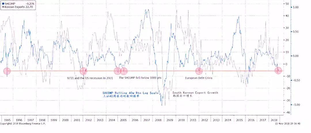
The trade war has been pressuring the Chinese stock market. As the instigator of the trade war, the US market hasn’t really felt the impact- till recently after China’sslowdown became more palpable. The question is: after plunging more than 30% and ranking among the worst-performing markets this year, has the Chinese market priced in the impact from the trade war?
To answer this question, we measure the rolling 40-week log-scale return of the Shanghai Composite. We would like to see how the magnitude of Shanghai’s plunge in 2018 compares with other periods of market trough. We can show that, after the selloff in 2018, this return measure has fallen to a level last seen during the 2001 US recession, during2005 when the Shanghai Composite fell below 1,000, as well as during the 2011 European sovereign debt crisis. That said, the return experienced during the 2008 global financial crisis and during the burst of the Chinese market bubble in 2015 is significantly more negative (
Figure 1
). As such, unless the trade war takes a wrong turn for the worse next year, the recent market price has largely reflected the near-term impact from the trade war, as well as economic slowdown.
Figure 1: The d
epressed market re
turn suggests the impact of trade war is largely priced in.
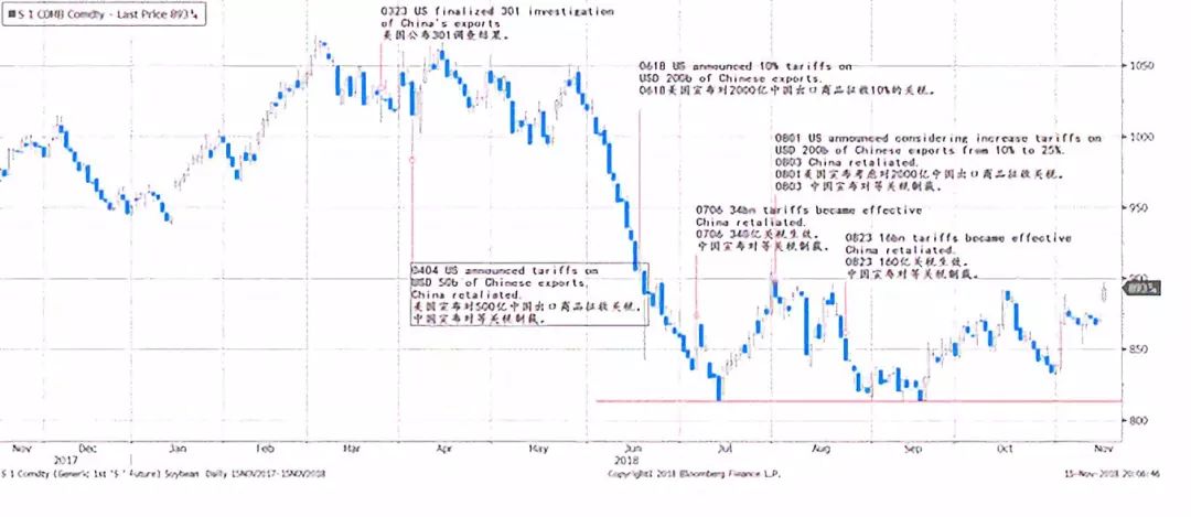
Another way to investigate the impact of the trade war is to look at the price of soybean futures – a commodity directly affected by the trade war due to its importance in US exports to China, as well as the Midwest’s sway in the US election. We note that the price of US soybean futures has stopped making new lows in recent months, even as the prospects of the trade war worsen (
Figure 2
). This observation shows that the market has largely priced in the near-term impact of the trade war. Both the Shanghai Composite and the US soybean futures are hinting at the likelihood of a truce in terms of market price for now. It is constructive that both sides are starting to talk again.
Figure 2: The price of US soybean futures has not made new lows.
TWO: Three Balance Sheets in China’s Economy
Our economic cycle model shows that China’sshort economic cycle will likely trough in the coming months, given the right mix of fiscal stimulus and monetary easing. Our cycle model also shows that theUS short economic cycle is peaking, and will likely continue to stir overseas markets in the near term (please refer to our report “
T
he Colliding Cycles of China and the US
” on 20180903).
When the economic cycle is approaching its upturning point, it means that the pendulum of negativity in the economy has swung too far. At this point, one can observe that credit expansion has slowed to a level below the nominal economic growth, despite falling interest rate; economic activities, notably building construction in China, are grinding to a halt; consumption is weak and inventory level is low. The stock market, one of the most watched barometers of economic activities, is depressed. China is now at this juncture.
However, for an economic cycle to turn up, help from government policy is often required. And the greater the challenges, the higher the intensity of policy support should be – as now. The condition for the policies to be effective, is that the government still has leeway to stimulate, and the private sector’s balance sheet is not leveraged to a point that is beyond repair. In short, there should still be room to transfer the burden of leverage between the public and private balance sheets.
In the following sections, we investigate the state of leverage in different parts of China’s economy.
Household: China’s Prope
rty Bubble – A Different Perspective
Is China’s property a bubble? This debate has not been settled - yet. Critics, including myself, have been applying extremely low rental yields versus mortgage rate,
high
ratio of property price to income and vacancy rate to justify their view of a property bubble. Yet, China’s property price continues to surge, despite these elaborate and thoughtful arguments. Although
property
is an asset of long duration and thus it is difficult to time the exit, such price performance suggests that the prevailing arguments may be too early to be right.
As the Chinese economy decelerates, and pressure on property price becomes increasingly palpable, the focus of the debate has turned to whether high property price has obliged Chinese households to take on leverage to an unsustainably high level, and has affected consumption. And eventually, such unsustainable leverage may lead to a bust of the property bubble.
Besides the conventional metrics of measuring housing affordability and the health of household balance sheet, we believe that it is more pertinent to check the debt service ratio of Chinese households over time and on a regional basis. The logic is that if the Chinese households can service their mortgage, then as long as
return
on property purchase exceeds mortgage rate, it is indeed rational to take on leverage. And as the property market varies between regions, it pays to look at regional differences.
Figure 3: 35 cities’
disposable income
outpacing mortgage payment
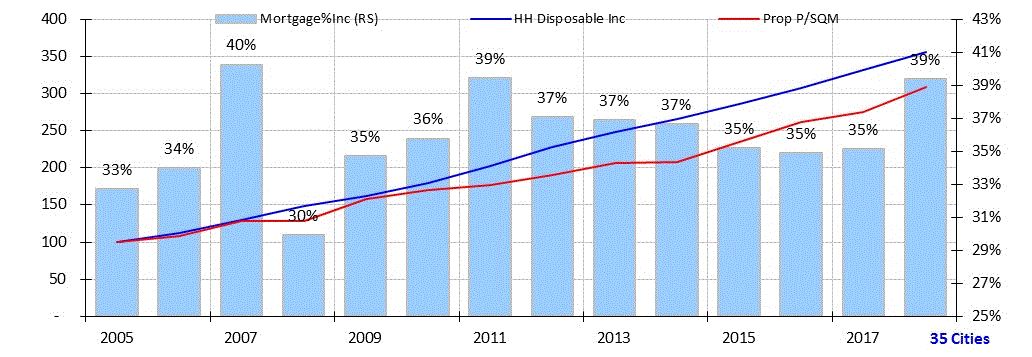
We find that, on a national level, household disposable income had outpaced property price appreciation. Mortgage payment as a percentage of household income is 39%. This ratio has risen to close to the highest level last seen in 2007 and 2011 – both followed by difficult years for China’s economy (
Figure 3
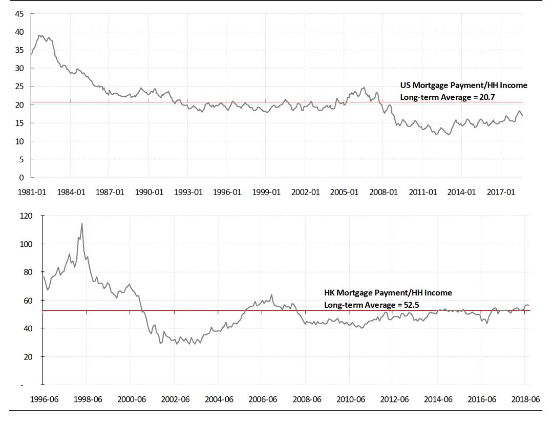
). Compared with 21% in the US where
interest
rate is starting to rise from historic lows, this ratio may suggest that the Chinese households are heavily in debt. But it compares favorably with that of Hong Kong at 56%, and Hong Kong’s ratio was higher than 100% during the bubble years of 1997. As such, there appears to be a cultural difference between the east and the west (
Figure 4
).
Fig
ure 4: HK/US
mortgage payment
as a percentage of income
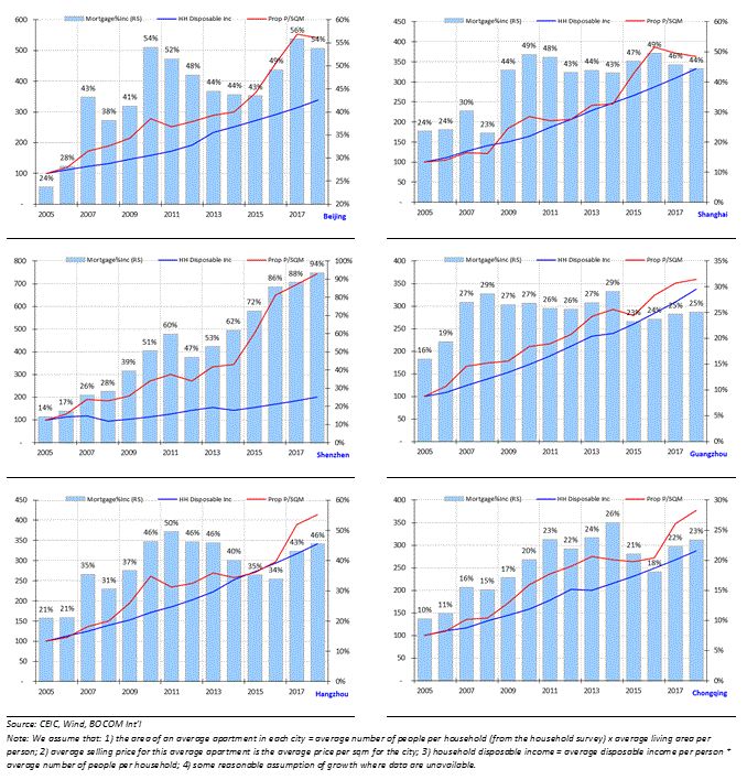
We apply the same methodology to calculate the mortgage service ratios of 35 major Chinese cities, with some reasonable assumptions (
Figure 5
shows a sample of cities; for presentation purpose, the rest please refer to
appendix
at the back of this report). We find that only 16 out of 35 major cities have seen household disposable income rising faster than property price since 2005. And all Tier-1 cities except Guangzhou have experienced faster property price growth than that of household income, respectively. That is, on a regional basis, the Chinese property bubble is
concerning,
if such trends persist.
Figure 5: Mortgage payment as % HH disposable income (6 cities sample; complete set in appendix)
In sum, we conclude that the Chinese households’ ability to service their mortgages has deteriorated to the level similar to 2007 and 2011, two of the years followed by difficult property market conditions in 2008 and 2012. These years also coincide with the last year of the short economic cycle in the US, which we will discuss later in the report. As a whole, the Chinese households’ balance sheet is highly leveraged, but is not yet on the brink of collapse – judging from the mortgage service ability.
Local Government Debt Woes
Can local governments go on with their increasing debt load? It has been a pesky concern for investors. Local government debt problems first surfaced in 2010, after the four-trillion-yuan stimulus in 2009. I still remember leading an investor group to conduct due diligence on local governments up and down the Yangtze back then. Recently, with headlines such as some counties failing to pay public servants’ stipends, the concerns on local government debts grow louder.
The challenge of analyzing local government debt lies in its transparency. Reliable data are hard to come by. And the LGFV and hidden liabilities via implicit debt guarantee for companies owned by or associated with local governments present further complications.
Our methodology is to use the bond data, of both local government bonds and the LGFV debt, to aggregate the apparent liabilities of local governments from bottom up. Such data include principal maturity and periodical interest payment information. We then compare these aggregated numbers with the numbers in sporadic news and national audits to verify their legitimacy. Obviously, our analysis does not include the implicit liabilities aforementioned. As the fiscal deficit on the central government level is still considered low at 2.7%, versus the international standard of 3%, we can save time by focusing on the local governments. We consider our analysis the best-case scenario analysis, as it includes only apparent liabilities and ignores potential new issuance from now (
Figure 6
).
We find that local governments’ ability to service debt, after deducting its responsibilities of fixed expenditures such as providing public security and education, will be tipped to negative in 2019. But it will deteriorate significantly in 2H2020, as the large
amount of bonds issued in the past three years come due.
We can assume that these bonds will be rolled over when they mature in 2020. But such a maneuver will increase local governments’ leverage even further. If we assume all these bonds can be paid off by transfer payments from the central government, it will increase central fiscal deficit to close to 4%.
If we assume all bonds maturing will be rolled over by issuing new debt, then the picture of local government debt service ability will improve greatly. Even so, local governments will still find it difficult to finance its liabilities in 2H2020. Either way, it is a monumental challenge. Fortunately, it is not yet an immediate threat.
Figure 6: Local government debt
service ability
will deteriorate significantly in 2H2020


Source: Wind, CEIC, BOCOM Int'l
Note:
1) We calculate local government liabilities by aggregating
both individual
local government bonds and LGFV debts outstanding. We note that
the headline
numbers are in general consistent with the numbers contained in
public news
. But our annual new bond issuance number is much larger than news data
, although
total issuance that is the sum of
new
bond plus replacement is
the same
. We believe our numbers are more reasonable, as the smaller numbers of
new issuance
according to news source would not have resulted in increasing
local government
debt outstanding. 2) Our local government revenue includes
transfer payments
from the central government and land sales, minus fixed expenditures
, including
public security, education etc.
Corporate Leverage Problems
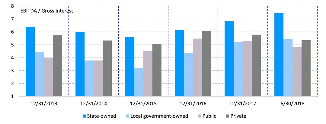
Recently, concerns have arisen over potential “fall-back” of private companies in China to state ownership, if the market turmoil continues. Many critics point to the diverging financial performances between state-owned and private enterprises in the manufacturing sector as the evidence of the malaise that private firms are suffering.
While these concerns are not without their merits, the manufacturing sector is only one part of the Chinese economy that is restructuring towards a consumption-led economy. Further, SOEs have natural advantages in this capital-intensive sector consisting of many upstream commodity producers. These sectors have strengthened during the supply-side reform. As such, using only the developments in the manufacturing sectors is tantamount to taking a few trees for the forest.
Once again, we analyze public companies’ debt service ability by measuring their EBITDA-Net interest coverage ratio. We aggregate public companies’ financial data from bottom up, and group them by ownership structure. Indeed, we find that the ability of state-owned and local government-owned companies to service debt has improved in the past five years, while that of private companies has deteriorated somewhat. That said, the net interest coverage ratio is still reasonable for private companies (
Figure 7
).
Recently, there have been concerns about the selling pressure induced by share pledge loans. Our quantitative analysis shows that the amount of shares pledged and the percentage of total market capitalization pledged have been rising since early 2015; even the stock market bubble burst only managed to put a fleeting dent in the share-pledge practice. The percentage of the market cap pledged had risen until March 2018, and then began to fall sharply. It appears that, as the market plunge accelerated, margin calls on shares pledged increased – it was like stepping on the gas pedal.
That said, given that the entire emerging market has been under pressure since late January, and that the percentage of market cap pledged has been rising in tandem as the market recovered from the 2015 crash, it is unlikely that these share-pledged loans are the reason for the bear market, although they must have aggravated it. Meanwhile, the surging volatility in the US market has not helped – the consequence of the colliding economic down-cycle in China and the peaking cycle in the US. We will discuss these cycles in the later section of this report.
Figure 7: EBITDA to net interest ratio of public companies by ownership
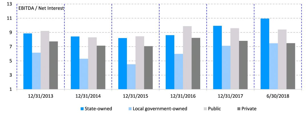
Source: Wind, BOCOM Int’l
Note :
1) Not all companies have data available. From 3,551 public-
listed companies
, we screen for 2,434 companies with consistent data availability.
Survivorship bias
may be present in this analysis. 2) We took out companies with no data
on interest
expense. These could be the weaker companies in the group. As such
, our
analysis can suffer from survivorship bias. 3) We then group them
by ownership
structure.
THREE: The Short Cycles of the US and China
“The only thing we learn from history is that we learn nothing from history.” – Hegel
The most pressing question
There exist a 3.5-year cycle in the US economy (
Figure 8
), and a 3-year cycle in China. We demonstrate in this paper as follows, with charts drawn from quantitative analysis, the cyclical character of the economies of the US and China.
After we published our first paper on economic cycles with quantitative metrics titled “
A Definitive Guid
e to China’s Economic Cycle
” (20170323), we were invited to give a public lecture on economic cycles at one of the most prestigious Chinese universities. A renowned economist, one of the finest of his kind, quipped: “Can you trade on it? How could you be sure that it will be the same next time?”
Forecast is hard, especially when it is about the future. While all models are wrong, some are useful. The significance of any cyclical model is to evaluate and forecast the underlying trend less perceptible to many, as well as the approximate timing of turning points. Such forecasts, albeit with no guarantee, improve the odds of profiting. Incidentally, we based our bearish 2018 outlook report titled “
View from the Peak
” (20171207) on the declining phase in China’s 3-year cycle - amid the then generally rosy consensus. Since its late January peak, the Shanghai Composite has fallen ~30%. Now the pressing question is: where is the bottom?
Figure 8: The short cycles in the US vs. P/E of the Shanghai Composite; the US short cycle has peaked
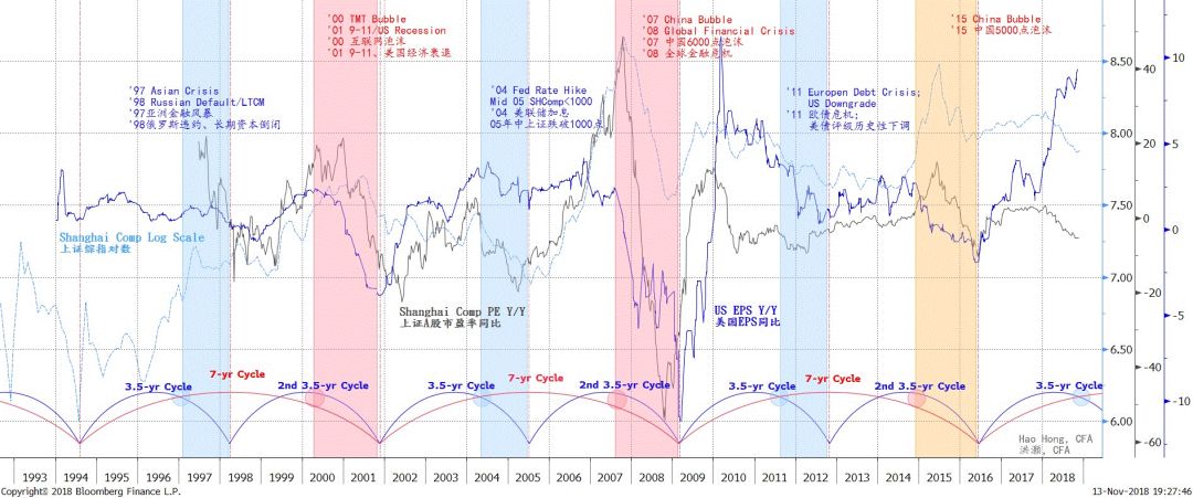
Source: Bloomberg, BOCOM Int’l
Note: Blue and red-shaded periods denote periods of downturn during the short(3.5-year) and intermedia (7-year) cycles of S&P 500 companies’ EPS (blue line), with blue periods being the mid-cycle slowdown and the red periods being the end of the 7-year cycle. The points where the short cycle crosses below the intermediate cycle are marked by blue circles. The points where both short and intermediate cycles start to turn down are marked by red circles. In the charts that follow, we use actual economic data to calculate precisely the ebbs and flows of the US cycles.
The short cycle in the US
“When in economics
we speak of cycles, we generally mean seven to eleven-year business cycles … which we shall agree to call ‘intermediate’, the existence of still shorter waves of about three and one-half years length has recently been shown to be probable... The length of the latter (intermediate waves) fluctuates at least between 7 and 11 years.” – The Long Waves in Economic Life, Nikolai D. Kondratieff
In
Figure 8
, we use the adjusted EPS of the S&P500 index as a proxy for the short-term fluctuations in the US economy. Our chart analysis shows that there clearly exists a 3.5-year cycle in the US economy. And two 3.5-year short cycles constitute a complete, trough-to-trough,7-year intermediate cycle. We observe the following in
Figure 8
:
(1)There have been six 3.5-year short cycles and three 7-year intermediate cycles since1994 (shown by blue and red arcs along the time axis at the chart bottom). Two of the most recent complete cycles run from Dec 2001 to Dec 2008, and from Dec2008 to Dec 2015, with mid-2005 and mid-2012 as the cyclical interludes, respectively.
(2)In the first 3.5-year short cycle within the 7-year intermediate cycle, when the short cycle finishes its uptrend and then crosses below the intermediate cycle(marked by blue circles), regional crises tend to be concurrent (shown and annotated in blue-shaded periods). For instance, the ’97 Asian Crisis and ’98Russian Defaults, and the European Sovereign Debt Crisis and the historic USsovereign rating downgrade in 2011. The current crises in Turkey and Argentina appear to be mid-cycle crises of such nature.
(3)In the second half of the 7-year intermediate cycle, when both the 3.5-year short cycle and the 7-year intermediate cycle start to decline (marked by red circles), crises of a more significant scale tend to happen. For instance, the burst of the TMT Bubble in 2000, the September-11 and the US recession in 2001, as well as the 2008 Global Financial Crisis (shown and annotated in red-shaded periods). Although much less discussed, the decline in the US stock market in2001 and 2008 are of similar magnitude – both had halved. These two episodes give us reasonable anchor in time to calculate the duration of the cycles. The positive influence the rising trends have on asset prices tends to last longer than the negative impact of the falling trends.
(4)History suggests that the snag that global markets are experiencing can be the last leg of an 11-year intermediate cycle consisting three 3.5-year short cycles starting from early 2009 and ending in early 2019. But it could also be the first 3.5-year short cycle within a renewed intermediate cycle of 7 years, consisting of two 3.5-year cycles and starting from early 2016. If so, the emerging turbulence ahead will bear much less significance than the end of an 11-year intermediate cycle would suggest.
(5)China’s own 3-year economic cycle is entering its last phase of decline in the coming months. This declining phase in the Chinese cycle happens to coincide with the late cycle in the US 3.5-year short cycle between 4Q18 and 1Q19, as suggested by our model (we will update our model on the Chinese economic cycle in the later part of this report). Expect significant turbulence. This coincidence can well be the reason why the Chinese stock market has been finding it hard to bottom out, albeit having cheapened substantially.
We charted
Figure 8
using the Bloomberg charting tools. While intuitive and visually appealing, we need to verify its rigor with quantitative
modelling. From
Figure 9
to
11
, we use monthly-adjusted EPSto model the short and intermediate cycles in the US economy. We can demonstrate clearly the 3.5-year short cycle, and the 7-year intermediate cycle consisting of two 3.5-year short cycles in the US economy for over two decades in the past.
We then overlay other US macroeconomic variables, such as the S&P 500 index, IP, capacity utilization, Leading Economic Indicator, capex plan and employment, with our US Cycle Indicator. Readers can see the very tight correlation between these variables and the Cycle Indicator.
Note that these correlations amongst market price, output, volume or surveys testify the validity of our cyclical model: the cycles identified here cannot be simply dismissed as happenstances. All of these important time series exhibit well-defined time duration of similar length. And their important turning points largely correspond, despite the complicated statistical and mathematical treatments of these data.
Deviation from general rules that prevails in the sequence of the cycles is very rare. Even when there is deviation from the underlying trend, such deviation tends to accelerate or retard its own momentum, rather than that of the underlying trends. The absence of such deviation is also are markable proof of the cycle’s existence.
Indeed, the 3.5-year short cycle in the US economy is consistent with the 3-year cycle in China’s economy that we identified in our previous report titled “
A definitive guide to China’s Economic Cycle
”
(20170323). The intermediate cycles of six to seven years consisting of two short cycles in these two economies are also consistent. These entwining short and intermediate cycles between the US andChina must have profound implications on economic and market performances, as well as policy choices.
Figure 9: The short cycles in the US (calculation based) vs. S&P 500; the US short cycle has peaked

Source: Bloomberg, BOCOM Int’l
Note: Blue and red-bracketed periods denote periods of downturn during the short
(3.5-year) and intermedia (7-year) cycle
s of S&P 500 companies’ EPS(blue line), with blue periods being the mid-cycle slowdown and the red periods being the end of the 7-year cycle.
Empirical e
vidence and policy implications
In afore and later discussions, we have defined with econometrics the 3.5-year and the 3-year short cycles in the US and China. These short cycles ebb and flow with regularity, as we observe similarity and simultaneity of fluctuations across various macroeconomic variables and across countries. The cycles seem to be fluctuating rhythmically around its underlying trend. We would not worry about the difference in duration of two quarters between the short cycles in the US and China, as cycles are not supposed to work with the precision of a quartz alarm clock.
In his seminal work “The Long Waves in Economic Life”, Kondratieff discussed the difference between the short/intermediate cycle and the long wave. He seemed to disagree with critics who believed that the short to intermediate cycles arose from the capitalistic system conditioned by “casual, extra-economic circumstances and events, such as: (1) changes in technology; (2) wars and revolution; (3) the assimilation of new countries into the world economy; and (4) fluctuations in gold production.” Instead, he believed that these changes that might appear to have altered the course of history were indeed endogenous to the cycles.
For instance, technological advances could have been made years before the turning points in the cycles, but could not be put to productive use given unfavorable economic conditions; war and revolution arose as the consequence of vying for scarce resources; with the old world growing and desiring for new markets came the assimilation of the new world; and the increase in gold production has been a result of rising monetary demand from economic expansion.
These conjectures, with well-argued reasons and empirical observations, help put the experiences in recent years into perspectives. The PBoC’s liquidity release for reconstruction of shanty towns in 2014, the Chinese market bubble in 2015, Trump’s presidential election win in 2016 and China’s supply-side reform, the subsequent revival of commodity prices since 2016 and the raging trade war are all endogenous to the “capitalistic system”. While the profound impact of these historic events had rippled through the markets, different supply-demand dynamics during different phases of economic cycles and their subsequent impact on market prices must have been conducive to the observation of these events. And the fluctuation in sentiment concurrent with market prices might have drawn our attention to these occurrences.
If so, as the US 3.5-year short cycle rising to its strength before the inflection point to fall below the 7-year intermediate cycle, it is likely to sway Mr. Trump’s decisions regarding the trade war to an even tougher stance, and eventually lead to a correction in the US market that appears to be going from strength to strength on the outside. Further, such inflection in the US short cycle can come as a surprise to the bullish market consensus, leading to a sudden and significant correction. Eventually, the deceleration phase in China’s 3-year short cycle will lead the US economy down.
Figure 10: The US short cycles(calculated) vs. various economic variables; the US shor
t cycle has peaked
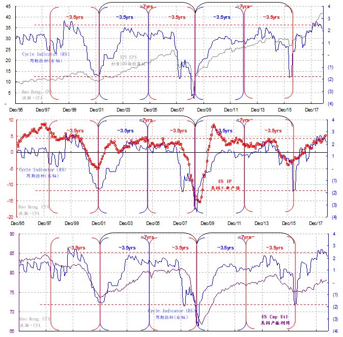
Figure 11: The US short cycles(calculated) vs. various economic variables; the US short cycle has peaked


