(点击
上方公众号
,可快速关注)
英文:jared polivka
翻译:
伯乐在线 - ggspeed
如有好文章投稿,请点击 → 这里了解详情
Galvanize 数据科学课程包括了一系列在科技产业的数据科学家中流行的机器学习课题,但是学生在 Galvanize 获得的技能并不仅限于那些最流行的科技产业应用。例如,在 Galvanize 的数据科学强化课中,音频信号和音乐分析较少被讨论,却它是一个有趣的机器学习概念应用。借用 Galvanize 课程中的课题,本篇教程为大家展示了如何利用 K-means 聚类算法从录音中分类和可视化音调,该方法会用到以下几个 python 工具包: NumPy/SciPy, Scikit-learn 和 Plotly。
K-means 聚类是什么
k-means 聚类算法是基于未标识数据集将相关项聚类的常用技术。给定 K 值后,该算法会将每个数据点划分到离其最近的中心点对应的簇,从而将整个数据集分成 k 组。k-means 算法有很广泛的应用,比如识别手机发射塔的有效位置,或为制造商选择服装的型号。而本教程将会为大家展示如何应用 k-means 根据音调来给音频分类。
音调的简单入门
一个音符是一串叠加的不同频率的 Sine 型波,而识别音符的音调需要识别那些听上去最突出的 Sine 型波的频率。
最简单的音符仅包含一个 Sine 型波:
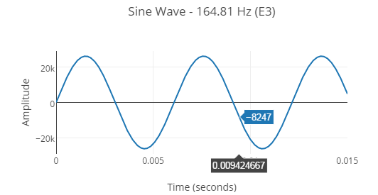

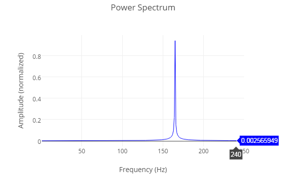
绘制的强度图谱中,每个组成要素频率的大小显示了上面波形的一个单独的频率。
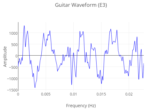
主流乐器制造出来的声音是由很多 sine 型波元素构成的,所以他们比上面展示的纯 sine 型波听起来更复杂。同样的音符(E3),由吉他弹奏出来的波形听看起来如下:
它的强度图谱显示了一个更大的基础频率的集合:
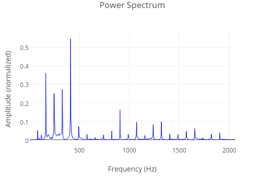
k-means 可以运用样例音频片段的强度图谱来给音调片段分类。给定一个有 n 个不同频率的强度图谱集合,k-means 将会给样例图谱分类,从而使在 n 维空间中每个图谱到它们组中心的欧式距离最小。
使用Numpy/SciPy从一个录音中创建数据集
本教程将会使用一个有 3 个不同音调的录音小样,每个音调是由吉他弹奏了 2 秒。
运用 SciPy 的 wavfile 模块可以轻松将一个 .wav 文件 转化为 NumPy 数值。
import
scipy
.
io
.
wavfile
as
wav
filename
=
'Guitar - Major Chord - E Gsharp B.wav'
# wav.read returns the sample_rate and a numpy array containing each audio sample from the .wav file
sample_rate
,
recording
=
wav
.
read
(
filename
)
这段录音应该被分为多个小段,从而使每段的音调都可以被独立地分类。
def
split_recording
(
recording
,
segment_length
,
sample_rate
)
:
segments
=
[]
index
=
0
while
index
<
len
(
recording
)
:
segment
=
recording
[
index
:
index
+
segment_length
<
em
>
sample_rate
]
segments
.
append
(
segment
)
index
+=
segment_length
em
>
sample_rate
return
segments
segment_length
=
.
5
# length in seconds
segments
=
split_recording
(
recording
,
segment_length
,
sample_rate
)
每一段的强度图谱可以通过傅里叶变换获得;傅里叶变换会将波形数据从时间域转换到频率域。以下的代码展示了如何使用 NumPy 实现傅里叶变换(Fourie transform)模块。
def
calculate_normalized_power_spectrum
(
recording
,
sample_rate
)
:
# np.fft.fft returns the discrete fourier transform of the recording
fft
=
np
.
fft
.
fft
(
recording
)
number_of_samples
=
len
(
recording
)
# sample_length is the length of each sample in seconds
sample_length
=
1.
/
sample_rate
# fftfreq is a convenience function which returns the list of frequencies measured by the fft
frequencies
=
np
.
fft
.
fftfreq
(
number_of_samples
,
sample_length
)
positive_frequency_indices
=
np
.
where
(
frequencies
>
0
)
# positive frequences returned by the fft
frequencies
=
frequencies
[
positive_frequency_indices
]
# magnitudes of each positive frequency in the recording
magnitudes
=
abs
(
fft
[
positive_frequency_indices
])
# some segments are louder than others, so normalize each segment
magnitudes
=
magnitudes
/
np
.
linalg
.
norm
(
magnitudes
)
return
frequencies
,
magnitudes
一些辅助函数会创建一个空的 NumPy 数值并将我们的样例强度图谱放入其中。
def
create_power_spectra_array
(
segment_length
,
sample_rate
)
:
number_of_samples_per_segment
=
int
(
segment_length
*
sample_rate
)
time_per_sample
=
1.
/
sample_rate
frequencies
=
np
.
fft
.
fftfreq
(
number_of_samples_per_segment
,
time_per_sample
)
positive_frequencies
=
frequencies
[
frequencies
>
0
]
power_spectra_array
=
np
.
empty
((
0
,
len
(
positive_frequencies
)))
return
power_spectra_array
def
fill_power_spectra_array
(
splits
,
power_spectra_array
,
fs
)
:
filled_array
=
power_spectra_array
for
segment
in
splits
:
freqs
,
mags
=
calculate_normalized_power_spectrum
(
segment
,
fs
)
filled_array
=
np
.
vstack
((
filled_array
,
mags
))
return
filled_array
power_spectra_array
=
create_power_spectra_array
(
segment_length
,
sample_rate
)
power_spectra_array
=
fill_power_spectra_array
(
segments
,
power_spectra_array
,
sample_rate
)
“power_spectra_array “是我们的训练数据集,它包含了一个强度图谱,在此图谱中录音按每 0.5 秒的间隔进行了分段。
利用 Scikit-learn 来执行 k-means
Scikit-learn 有一个易用的 k-means 实现。我们的音频样例包括 3 个不同的音调,所以将 k 设置为 3。
from
sklearn
.
cluster
import
KMeans
kmeans
=
KMeans
(
3
,
max
<
em
>
iter
=
1000
,
n_init
=
100
)
kmeans
.
fit_transform
(
power_spectra_array
)
predictions
=
kmeans
.
predict
(
power_spectra_array
)
“predictions”是一个 Python 数据,它包含了 12 个音频分段的分组标签(一个任意的整数)。
print
predictions
=>
[
2
2
2
2
0
0
0
0
1
1
1
1
]
这个数组说明了在听这段音频时连续音频分段被正确地分在了一起。
使用 Plotly 可视化结果
为了更好的理解预测结果,需要绘制每个样例的强度图谱,每个样例均用颜色来标记出其对应的 k-means 分组结果。
# find x-values for plot (frequencies)
number
<
em
>
of_samples
=
int
(
segment_length
*
sample_rate
)
sample_length
=
1.
/
sample_rate
frequencies
=
np
.
fft
.
fftfreq
(
number_of_samples
,


