We review the math and code needed to fit a Gaussian Process (GP) regressor to data. We conclude with a demo of a popular application, fast function minimization through GP-guided search. The gif below illustrates this approach in action — the red points are samples from the hidden red curve. Using these samples, we attempt to leverage GPs to find the curve’s minimum as fast as possible.
Appendices contain quick reviews on (i) the GP regressor posterior derivation, (ii) SKLearn’s GP implementation, and (iii) GP classifiers.
Follow @efavdb
Follow us on twitter for new submission alerts!
Introduction
Gaussian Processes (GPs) provide a tool for treating the following general problem: A function $f(x)$ is sampled at $n$ points, resulting in a set of noisy$^1$ function measurements, $\{f(x_i) = y_i \pm \sigma_i, i = 1, \ldots, n\}$. Given these available samples, can we estimate the probability that $f = \hat{f}$, where $\hat{f}$ is some candidate function?
To decompose and isolate the ambiguity associated with the above challenge, we begin by applying Bayes’s rule,
\begin{eqnarray} \label{Bayes} \tag{1}
p(\hat{f} \vert \{y\}) = \frac{p(\{y\} \vert \hat{f} ) p(\hat{f})}{p(\{y\}) }.
\end{eqnarray}
The quantity at left above is shorthand for the probability we seek — the probability that $f = \hat{f}$, given our knowledge of the sampled function values $\{y\}$. To evaluate this, one can define and then evaluate the quantities at right. Defining the first in the numerator requires some assumption about the source of error in our measurement process. The second function in the numerator is the prior — it is here where the greatest assumptions must be taken. For example, we’ll see below that the prior effectively dictates the probability of a given smoothness for the $f$ function in question.
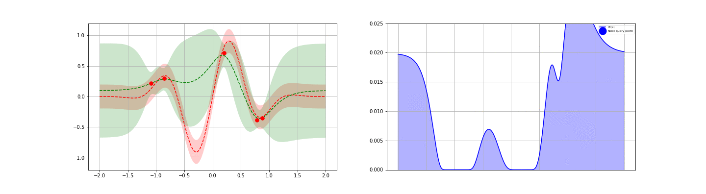
In the GP approach, both quantities in the numerator at right above are taken to be multivariate Normals / Gaussians. The specific parameters of this Gaussian can be selected to ensure that the resulting fit is good — but the Normality requirement is essential for the mathematics to work out. Taking this approach, we can write down the posterior analytically, which then allows for some useful applications. For example, we used this approach to obtain the curves shown in the top figure of this post — these were obtained through random sampling from the posterior of a fitted GP, pinned to equal measured values at the two pinched points shown. Posterior samples are useful for visualization and also for taking Monte Carlo averages.
In this post, we (i) review the math needed to calculate the posterior above, (ii) discuss numerical evaluations and fit some example data using GPs, and (iii) review how a fitted GP can help to quickly minimize a cost function — eg a machine learning cross-validation score. Appendices cover the derivation of the GP regressor posterior, SKLearn’s GP implementation, and GP Classifiers.