(点击
上方蓝字
,快速关注我们)
编译:伯乐在线 - JLee
如有好文章投稿,请点击 → 这里了解详情
第3节:分层模型
贝叶斯模型的一个核心优势就是简单灵活,可以实现一个分层模型。这一节将实现和比较整体合并模型和局部融合模型。
import
itertools
import
matplotlib
.
pyplot
as
plt
import
numpy
as
np
import
pandas
as
pd
import
pymc3
as
pm
import
scipy
import
scipy
.
stats
as
stats
import
seaborn
.
apionly
as
sns
from
IPython
.
display
import
Image
from
sklearn
import
preprocessing
%
matplotlib
inline
plt
.
style
.
use
(
'bmh'
)
colors
=
[
'#348ABD'
,
'#A60628'
,
'#7A68A6'
,
'#467821'
,
'#D55E00'
,
'#CC79A7'
,
'#56B4E9'
,
'#009E73'
,
'#F0E442'
,
'#0072B2'
]
messages
=
pd
.
read_csv
(
'data/hangout_chat_data.csv'
)
模型合并
让我们采取一种不同的方式来对我的 hangout 聊天回复时间进行建模。我的直觉告诉我回复的快慢与聊天的对象有关。我很可能回复女朋友比回复一个疏远的朋友更快。这样,我可以对每个对话独立建模,对每个对话i估计参数 μi 和 αi。μi=Uniform(0,100)
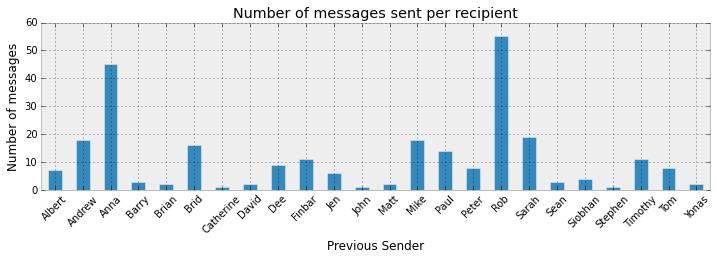
一个必须考虑的问题是,有些对话相比其他的含有的消息很少。这样,和含有大量消息的对话相比,我们对含有较少消息的对话的回复时间的估计,就具有较大的不确定度。下图表明了每个对话在样本容量上的差异。
ax
=
messages
.
groupby
(
'prev_sender'
)[
'conversation_id'
].
size
().
plot
(
kind
=
'bar'
,
figsize
=
(
12
,
3
),
title
=
'Number of messages sent per recipient'
,
color
=
colors
[
0
])
_
=
ax
.
set_xlabel
(
'Previous Sender'
)
_
=
ax
.
set_ylabel
(
'Number of messages'
)
_
=
plt
.
xticks
(
rotation
=
45
)
对于每个对话i中的每条消息j,模型可以表示为:

indiv_traces
=
{}
# Convert categorical variables to integer
le
=
preprocessing
.
LabelEncoder
()
participants_idx
=
le
.
fit_transform
(
messages
[
'prev_sender'
])
participants
=
le
.
classes_
n_participants
=
len
(
participants
)
for
p
in
participants
:
with
pm
.
Model
()
as
model
:
alpha
=
pm
.
Uniform
(
'alpha'
,
lower
=
0
,
upper
=
100
)
mu
=
pm
.
Uniform
(
'mu'
,
lower
=
0
,
upper
=
100
)
data
=
messages
[
messages
[
'prev_sender'
]
==
p
][
'time_delay_seconds'
].
values
y_est
=
pm
.
NegativeBinomial
(
'y_est'
,
mu
=
mu
,
alpha
=
alpha
,
observed
=
data
)
y_pred
=
pm
.
NegativeBinomial
(
'y_pred'
,
mu
=
mu
,
alpha
=
alpha
)
start
=
pm
.
find_MAP
()
step
=
pm
.
Metropolis
()
trace
=
pm
.
sample
(
20000
,
step
,
start
=
start
,
progressbar
=
True
)
indiv_traces
[
p
]
=
trace
Applied
interval
-
transform to alpha
and
added transformed alpha_interval to
model
.
Applied
interval
-
transform to mu
and
added transformed mu_interval to
model
.
[
-----------------
100
%-----------------
]
20000
of
20000
complete
in
9.7
secApplied
interval
-
transform to alpha
and
added transformed alpha_interval to
model
.
Applied
interval
-
transform to mu
and
added transformed mu_interval to
model
.
[
-----------------
100
%-----------------
]
20000
of
20000
complete
in
12.4
secApplied
interval
-
transform to alpha
and
added transformed alpha_interval to
model
.
Applied
interval
-
transform to mu
and
added transformed mu_interval to
model
.
[
-----------------
100
%-----------------
]
20000
of
20000
complete
in
12.0
secApplied
interval
-
transform to alpha
and
added transformed alpha_interval to
model
.
Applied
interval
-
transform to mu
and
added transformed mu_interval to
model
.
[
-----------------
100
%-----------------
]
20000
of
20000
complete
in
12.0
secApplied
interval
-
transform to alpha
and
added transformed alpha_interval to
model
.
Applied
interval
-
transform to mu
and
added transformed mu_interval to
model
.
[
-----------------
100
%-----------------
]
20000
of
20000
complete
in
10.3
secApplied
interval
-
transform to alpha
and
added transformed alpha_interval to
model
.
Applied
interval
-
transform to mu
and
added transformed mu_interval to
model
.
[
-----------------
100
%-----------------
]
20000
of
20000
complete
in
16.4
secApplied
interval
-
transform to alpha
and
added transformed alpha_interval to
model
.
Applied
interval
-
transform to mu
and
added transformed mu_interval to
model
.
[
-----------------
100
%-----------------
]
20000
of
20000
complete
in
12.1
secApplied
interval
-
transform to alpha
and
added transformed alpha_interval to
model
.
Applied
interval
-
transform to mu
and
added transformed mu_interval to
model
.
[
-----------------
100
%-----------------
]
20000
of
20000
complete
in
17.4
secApplied
interval
-
transform to alpha
and
added transformed alpha_interval to
model
.
Applied
interval
-
transform to mu
and
added transformed mu_interval to
model
.
[
-----------------
100
%-----------------
]
20000
of
20000
complete
in
19.9
secApplied
interval
-
transform to alpha
and
added transformed alpha_interval to
model
.
Applied
interval
-
transform to mu
and
added transformed mu_interval to
model
.
[
-----------------
100
%-----------------
]
20000
of
20000
complete
in
15.2
secApplied
interval
-
transform to alpha
and
added transformed alpha_interval to
model
.
Applied
interval
-
transform to mu
and
added transformed mu_interval to
model
.
[
-----------------
100
%-----------------
]
20000
of
20000
complete
in
16.1
secApplied
interval
-
transform to alpha
and
added transformed alpha_interval to
model
.
Applied
interval
-
transform to mu
and
added transformed mu_interval to
model
.
[
-----------------
100
%-----------------
]
20000
of
20000
complete
in
10.1
secApplied
interval
-
transform to alpha
and
added transformed alpha_interval to
model
.
Applied
interval
-
transform to mu
and
added transformed mu_interval to
model
.
[
-----------------
100
%-----------------
]
20000
of
20000
complete
in
11.1
secApplied
interval
-
transform to alpha
and
added transformed alpha_interval to
model
.
Applied
interval
-
transform to mu
and
added transformed mu_interval to
model
.
[
-----------------
100
%-----------------
]
20000
of
20000
complete
in
11.9
secApplied
interval
-
transform to alpha
and
added transformed alpha_interval to
model
.
Applied
interval
-
transform to mu
and
added transformed mu_interval to
model
.
[
-----------------
100
%-----------------
]
20000
of
20000
complete
in
12.8
secApplied
interval
-
transform to alpha
and
added transformed alpha_interval to
model
.
Applied
interval
-
transform to mu
and
added transformed mu_interval to
model
.
[
-----------------
100
%-----------------
]
20000
of
20000
complete
in
13.0
secApplied
interval
-
transform to alpha
and
added transformed alpha_interval to
model
.
Applied
interval
-
transform to mu
and
added transformed mu_interval to
model
.
[
-----------------
100
%-----------------
]
20000
of
20000
complete
in
12.4
secApplied
interval
-
transform to alpha
and
added transformed alpha_interval to
model
.
Applied
interval
-
transform to mu
and
added transformed mu_interval to
model
.
[
-----------------
100
%-----------------
]
20000
of
20000
complete
in
10.9
secApplied
interval
-
transform to alpha
and
added transformed alpha_interval to
model
.
Applied
interval
-
transform to mu
and
added transformed mu_interval to
model
.
[
-----------------
100
%-----------------
]
20000
of
20000
complete
in
22.6
secApplied
interval
-
transform to alpha
and
added transformed alpha_interval to
model
.
Applied
interval
-
transform to mu
and
added transformed mu_interval to
model
.
[
-----------------
100
%-----------------
]
20000
of
20000
complete
in
18.7
secApplied
interval
-
transform to alpha
and
added transformed alpha_interval to
model
.
Applied
interval
-
transform to mu
and
added transformed mu_interval to
model
.
[
-----------------
100
%-----------------
]
20000
of
20000
complete
in
13.1
secApplied
interval
-
transform to alpha
and
added transformed alpha_interval to
model
.
Applied
interval
-
transform to mu
and
added transformed mu_interval to
model
.
[
-----------------
100
%-----------------
]
20000
of
20000
complete
in
13.9
secApplied
interval
-
transform to alpha
and
added transformed alpha_interval to
model
.
Applied
interval
-
transform to mu
and
added transformed mu_interval to
model
.
[
-----------------
100
%-----------------
]
20000
of
20000
complete
in
14.0
secApplied
interval
-
transform to alpha
and
added transformed alpha_interval to
model
.
Applied
interval
-
transform to mu
and
added transformed mu_interval to
model
.
[
-----------------
100
%-----------------
]
20000
of
20000
complete
in
13.6
sec
fig
,
axs
=
plt
.
subplots
(
3
,
2
,
figsize
=
(
12
,
6
))
axs
=
axs
.
ravel
()
y_left_max
=
2
y_right_max
=
2000
x_lim
=
60
ix
=
[
3
,
4
,
6
]
for
i
,
j
,
p
in
zip
([
0
,
1
,
2
],
[
0
,
2
,
4
],
participants
[
ix
])
:
axs
[
j
].
set_title
(
'Observed: %s'
%
p
)
axs
[
j
].
hist
(
messages
[
messages
[
'prev_sender'
]
==
p
][
'time_delay_seconds'
].
values
,
range
=
[
0
,
x_lim
],
bins
=
x_lim
,
histtype
=
'stepfilled'
)
axs
[
j
].
set_ylim
([
0
,
y_left_max
])
for
i
,
j
,
p
in
zip
([
0
,
1
,
2
],
[
1
,
3
,
5
],
participants
[
ix
])
:
axs
[
j
].
set_title
(
'Posterior predictive distribution: %s'
%
p
)
axs
[
j
].
hist
(
indiv_traces
[
p
].
get_values
(
'y_pred'
),
range
=
[
0
,
x_lim
],
bins
=
x_lim
,
histtype
=
'stepfilled'
,
color
=
colors
[
1
])
axs
[
j
].
set_ylim
([
0
,
y_right_max
])
axs
[
4
].
set_xlabel
(
'Response time (seconds)'
)
axs
[
5
].
set_xlabel
(
'Response time (seconds)'
)
plt
.
tight_layout
()
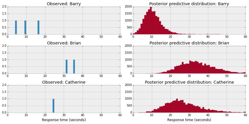
上图显示了3例对话的观测数据分布(左)和后验预测分布(右)。可以看出,不同对话的后验预测分布大不相同。这可能准确反映出对话的特点,也可能是样本容量太小造成的误差。
如果我们把后验预测分布联合起来,我们希望得到的分布和观测数据分布近似,让我们来进行后验预测检验。
combined_y_pred
=
np
.
concatenate
([
v
.
get_values
(
'y_pred'
)
for
k
,
v
in
indiv_traces
.
items
()])
x_lim
=
60
y_pred
=
trace
.
get_values
(
'y_pred'
)
fig
=
plt
.
figure
(
figsize
=
(
12
,
6
))
fig
.
add_subplot
(
211
)
fig
.
add_subplot
(
211
)
_
=
plt
.
hist
(
combined_y_pred
,
range
=
[
0
,
x_lim
],
bins
=
x_lim
,
histtype
=
'stepfilled'
,
color
=
colors
[
1
])
_
=
plt
.
xlim
(
1
,
x_lim
)
_
=
plt
.
ylim
(
0
,
20000
)
_
=
plt
.
ylabel
(
'Frequency'
)
_
=
plt
.
title
(
'Posterior predictive distribution'
)
fig
.
add_subplot
(
212
)
_
=
plt
.
hist
(
messages
[
'time_delay_seconds'
].
values
,
range
=
[
0
,
x_lim
],
bins
=
x_lim
,
histtype
=
'stepfilled'
)
_
=
plt
.
xlim
(
0
,
x_lim
)
_
=
plt
.
xlabel
(
'Response time in seconds'
)
_
=
plt
.
ylim
(
0
,
20
)
_
=
plt
.
ylabel
(
'Frequency'
)
_
=
plt
.
title
(
'Distribution of observed data'
)
plt
.
tight_layout
()
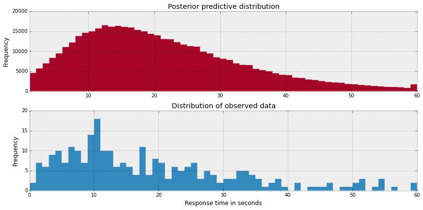
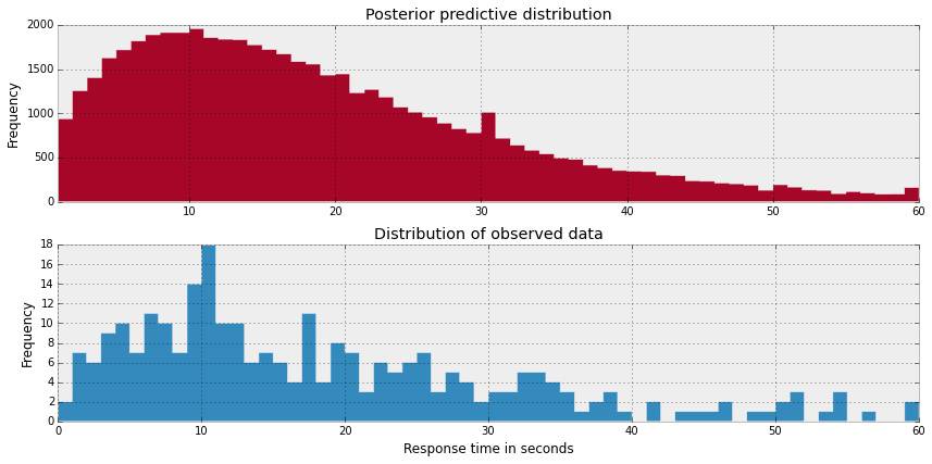
是的,后验预测分布和观测数据的分布近似。但是,我关心的是数据较少的对话,对它们的估计也可能具有较大的方差。一个减小这种风险的方法是分享对话信息,但仍对每个对话单独估计 μi,我们称之为局部融合。
局部融合
就像整体合并模型,局部融合模型对每个对话i都有独自的参数估计。但是,这些参数通过融合参数联系在一起。这反映出,我的不同对话间的response_time有相似之处,就是我本性上倾向于回复快或慢。

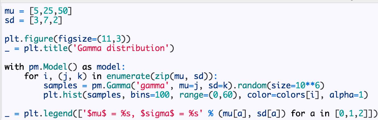
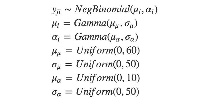
接着上面的例子,估计负二项分布的参数 μi 和 αi。相比于使用均匀分布作为先验分布,我使用带两个参数(μ,σ)的伽马分布,从而当能够预测 μ 和 σ 的值时,可以引入更多的先验信息到模型中。
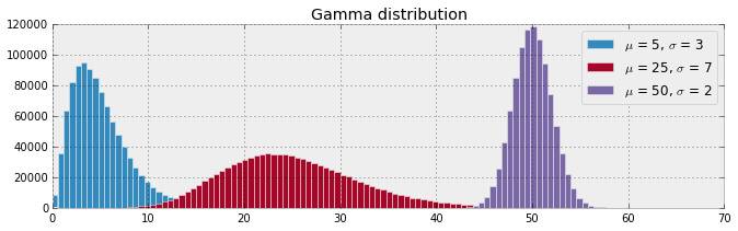
首先,我们来看看伽马分布,下面你可以看到,它非常灵活。
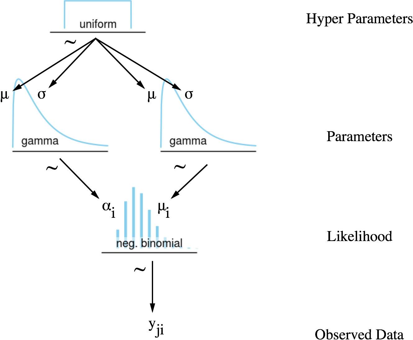
局部融合模型可以表示为:
代码:
Image('graphics/dag neg poisson gamma hyper.png', width=420)
with
pm
.
Model
()
as
model
:
hyper_alpha_sd
=
pm
.
Uniform
(
'hyper_alpha_sd'
,
lower
=
0
,
upper
=
50
)
hyper_alpha_mu
=
pm
.
Uniform
(
'hyper_alpha_mu'
,
lower
=
0
,
upper
=
10
)
hyper_mu_sd
=
pm
.
Uniform
(
'hyper_mu_sd'
,
lower
=
0
,
upper
=
50
)
hyper_mu_mu
=
pm
.
Uniform
(
'hyper_mu_mu'
,
lower
=
0
,
upper
=
60
)
alpha
=
pm
.
Gamma
(
'alpha'
,
mu
=
hyper_alpha_mu
,
sd
=
hyper_alpha_sd
,
shape
=
n_participants
)
mu
=
pm
.
Gamma
(
'mu'
,
mu
=
hyper_mu_mu
,
sd
=
hyper_mu_sd
,
shape
=
n_participants
)
y_est
=
pm
.
NegativeBinomial
(
'y_est'
,
mu
=
mu
[
participants_idx
],
alpha
=
alpha
[
participants_idx
],
observed
=
messages
[
'time_delay_seconds'
].
values
)
y_pred
=
pm
.
NegativeBinomial
(
'y_pred'
,
mu
=
mu
[
participants_idx
],
alpha
=
alpha
[
participants_idx
],
shape
=
messages
[
'prev_sender'
].
shape
)
start
=
pm
.
find_MAP
()
step
=
pm
.
Metropolis
()
hierarchical_trace
=
pm
.
sample
(
200000
,
step
,
progressbar
=
True
)
Applied
interval
-
transform to hyper_alpha_sd
and
added transformed hyper_alpha_sd_interval to
model
.
Applied
interval
-
transform to hyper_alpha_mu
and
added transformed hyper_alpha_mu_interval to
model
.
Applied
interval
-
transform to hyper_mu_sd
and
added transformed hyper_mu_sd_interval to
model
.
Applied
interval
-
transform to hyper_mu_mu
and
added transformed hyper_mu_mu_interval to
model
.
Applied
log
-
transform to alpha
and
added transformed alpha_log to
model
.
Applied
log
-
transform to mu
and
added transformed mu_log to
model
.
[
-----------------
100
%-----------------
]
200000
of
200000
complete
in
593.0
sec
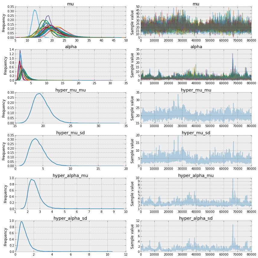
对 μ 和 α 的估计有多条曲线,每个对话i对应一条。整体合并和局部融合模型的不同之处在于,局部融合模型的参数(μ和 α)拥有一个被所有对话共享的融合参数。这带来两个好处:
-
信息在对话间共享,所以对于含有有限样本容量的对话来说,在估计过程中从别的对话处“借”信息来减小估计的方差。
-
我们对每个对话单独做了估计,也对所有对话整体做了估计。
我们快速看一下后验预测分布
x_lim
=
60
y_pred
=
hierarchical_trace
.
get_values
(
'y_pred'
)[
::
1000
].
ravel
()
fig
=
plt
.
figure
(
figsize
=
(
12
,
6
))
fig
.
add_subplot
(
211
)
fig
.
add_subplot
(
211
)
_
=
plt
.
hist
(
y_pred
,
range
=
[
0
,
x_lim
],
bins
=
x_lim
,
histtype
=
'stepfilled'
,
color
=
colors
[
1
])
_
=
plt
.
xlim
(
1
,
x_lim
)
_
=
plt
.
ylabel
(
'Frequency'
)
_
=
plt
.
title
(
'Posterior predictive distribution'
)
fig
.
add_subplot
(
212
)
_
=
plt
.
hist
(
messages
[
'time_delay_seconds'
].
values
,
range
=
[
0
,
x_lim
],
bins
=
x_lim
,
histtype
=
'stepfilled'
)
_
=
plt
.
xlabel
(
'Response time in seconds'
)
_
=
plt
.
ylabel
(
'Frequency'
)
_
=
plt
.
title
(
'Distribution of observed data'
)
plt
.
tight_layout
()
收缩效果:合并模型 vs 分层模型
如讨论的那样,局部融合模型中 μ 和 α 享有一个融合参数,通过对话间信息共享,它使得参数的估计收缩得更紧密,尤其是对含有少量数据的对话。
下图显示了这种收缩效果,可以看出通过融合参数,参数μ 和 α 是怎样聚集在一起。
hier_mu
=
hierarchical_trace
[
'mu'
][
500
:
].
mean
(
axis
=
0
)
hier_alpha
=
hierarchical_trace
[
'alpha'
][
500
:
].
mean
(
axis
=
0
)
indv_mu
=
[
indiv_traces
[
p
][
'mu'
][
500
:
].
mean
()
for
p
in
participants
]
indv_alpha
=
[
indiv_traces
[
p
][
'alpha'
][
500
:
].
mean
()
for
p
in
participants
]
fig
=
plt
.
figure
(
figsize
=
(
8
,
6
))
ax
=
fig
.
add_subplot
(
111
,
xlabel
=
'mu'
,
ylabel
=
'alpha'
,
title
=
'Pooled vs. Partially Pooled Negative Binomial Model'
,
xlim
=
(
5
,
45