专栏名称: YuLabSMU

专注于生物信息学、R语言和可视化，只有原创、拒绝爆款！

一文解决RT-PCR的统计分析

YuLabSMU · 公众号 · · 2018-01-18 08:00

正文

话说当年我在暨大工作的时候，学生都很害怕汇报RT-PCR的结果，因为每次一讲到用了t test做了检验，底下某小老板，就一顿狂喷，说学生瞎搞，这不对那不对，但从没告诉正确的姿势，学生们都怕了他。于是我写了这篇文章，普及了一下相关的知识，RT-PCR那点东西，全在这里。

RT-PCR相对定量有两个模型，一是 $Δ Δ C t$ 模型，一个是扩增效率校正模型。这里我们先讨论简单的模型： $Δ Δ C t$ 模型，在这一模型中，假定扩增效率为2，即每个PCR cycle，产物倍增，由以下公式给出：

$R a t i o = 2^{- Δ Δ C t}$

其中ΔΔC _t = ΔΔC _treated - ΔΔC _control , ΔΔC _treated 和ΔΔC _control 分别是treatment组和control组中目标基因和参照基因的Ct差，即ΔΔC _t = ΔΔC _target - ΔΔC _reference .

扩增效率肯定是在(1,2)之间，理想状态下才是2，而理想状态通常是不存在的。这个模型的假设点其实是treatment组和control组的扩增效率一样，至于是不是2，比2小多少，并不影响后续的统计分析。

Data

我们来看以下一份数据，4组重复实验，用RT-PCR测了gene01和gene02的表达量，HK代表house keeping gene，即参照。以下数值为原始的Ct值。

ct             sample = rep(rep(1:4, each=3), 2),
        treatment = rep(c("Control","Treated"), each=12),
        gene01 = c(23.22,23.34,23.12,24.06,24.15,24.15,23.18,23.13,
                    23.10,24.78,24.45,24.67,23.11,22.99,23.10,22.77,
                    22.99,23.06,23.73,24.01,23.80,23.73,23.83,23.73),
        gene02 = c(29.08,29.04,29.39,28.23,28.01,28.12,28.79,28.43,
                    28.49,31.37,30.74,31.09,27.11,27.24,27.37,25.52,
                    25.72,25.52,27.43,26.73,26.65,27.96,27.84,27.98),
        HK = c(19.68,19.69,19.80,19.95,19.93,19.97,19.93,20.02,20.27,
                    19.93,19.88,19.90,20.61,19.98,20.57,19.68,19.95,
                    19.85,20.27,20.08,20.07,20.10,20.07,20.10)
            )
print(ct)

##    sample treatment gene01 gene02    HK
## 1       1   Control  23.22  29.08 19.68
## 2       1   Control  23.34  29.04 19.69
## 3       1   Control  23.12  29.39 19.80
## 4       2   Control  24.06  28.23 19.95
## 5       2   Control  24.15  28.01 19.93
## 6       2   Control  24.15  28.12 19.97
## 7       3   Control  23.18  28.79 19.93
## 8       3   Control  23.13  28.43 20.02
## 9       3   Control  23.10  28.49 20.27




    

## 10      4   Control  24.78  31.37 19.93
## 11      4   Control  24.45  30.74 19.88
## 12      4   Control  24.67  31.09 19.90
## 13      1   Treated  23.11  27.11 20.61
## 14      1   Treated  22.99  27.24 19.98
## 15      1   Treated  23.10  27.37 20.57
## 16      2   Treated  22.77  25.52 19.68
## 17      2   Treated  22.99  25.72 19.95
## 18      2   Treated  23.06  25.52 19.85
## 19      3   Treated  23.73  27.43 20.27
## 20      3   Treated  24.01  26.73 20.08
## 21      3   Treated  23.80  26.65 20.07
## 22      4   Treated  23.73  27.96 20.10
## 23      4   Treated  23.83  27.84 20.07
## 24      4   Treated  23.73  27.98 20.10

Data clean

每个sample，测了三次技术重复，我们使用平均值来提高精度。

require(plyr)

## Loading required package: plyr
ct         data.frame(gene01=mean(x$gene01), 
            gene02=mean(x$gene02), HK=mean(x$HK)))
print(ct)

##   sample treatment   gene01   gene02       HK
## 1      1   Control 23.22667 29.17000 19.72333
## 2      1   Treated 23.06667 27.24000 20.38667
## 3      2   Control 24.12000 28.12000 19.95000
## 4      2   Treated 22.94000 25.58667 19.82667
## 5      3   Control 23.13667 28.57000 20.07333
## 6      3   Treated 23.84667 26.93667 20.14000
## 7      4   Control 24.63333 31.06667 19.90333
## 8      4   Treated 23.76333 27.92667 20.09000

Calculate statistical metric

按照ΔΔC _t 模型，我们先计算ΔC _t ，然后计算ΔΔC _t ，最终计算出Ratio。

delta.ct     data.frame(gene01=x$gene01-x$HK, 
            gene02=x$gene02-x$HK))
print(delta.ct)

##   sample treatment   gene01    gene02




    

## 1      1   Control 3.503333  9.446667
## 2      1   Treated 2.680000  6.853333
## 3      2   Control 4.170000  8.170000
## 4      2   Treated 3.113333  5.760000
## 5      3   Control 3.063333  8.496667
## 6      3   Treated 3.706667  6.796667
## 7      4   Control 4.730000 11.163333
## 8      4   Treated 3.673333  7.836667

## Delta Delta Ct
dd.ct     select=c(gene01, gene02)) - 
    subset(delta.ct, 
           treatment=="Control", 
           select=c(gene01, gene02))
print(dd.ct)

##       gene01    gene02
## 2 -0.8233333 -2.593333
## 4 -1.0566667 -2.410000
## 6  0.6433333 -1.700000
## 8 -1.0566667 -3.326667
ratio print(ratio)

##     gene01    gene02
## 2 1.769490  6.034915
## 4 2.080120  5.314743
## 6 0.640232  3.249010
## 8 2.080120 10.032899

这个ratio值计算出，经过扩增后，目的基因在处理组中的产量是对照组的多少倍。

Statistical Analysis

计算出ratio后，很多人就拿它来做t检验。这种做法是不对的，因为ratio的分布明显是右偏的。从理论上看，PCR的扩增可以分成以下三个阶段，指数扩增、线性扩增、平台期。

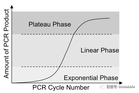
当试剂量足够的时候，就处于指数扩增阶段，只有当PCR试剂不足时，才进入线性扩增期，最后当试剂被耗尽时，产物不增长，位于平台期。

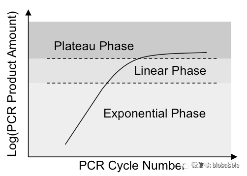
在我们的实验中，通常PCR反应是处于指数增长期。我们将其进行对数处理，指数增长就会变成线性增长，这样数据的右偏现象就会有明显减弱，当然我不敢说对数转换后，它就能呈正态分布，但起码对数处理后数据的分布比原始ratio数据更接近正态了。

T Test

只有偏态不明显的情况下，才可以用t检验进行分析。

## T test for gene01
t.test(log(ratio[,1], base=2), mu = 0)

## 
##  One Sample t-test
## 
## data:  log(ratio[, 1], base = 2)
## t = 1.4009, df = 3, p-value = 0.2558
## alternative hypothesis: true mean is not equal to 0




    

## 95 percent confidence interval:
##  -0.729139  1.875806
## sample estimates:
## mean of x 
## 0.5733333

## T test for gene02
t.test(log(ratio[,2], base=2), mu = 0)

## 
##  One Sample t-test
## 
## data:  log(ratio[, 2], base = 2)
## t = 7.5039, df = 3, p-value = 0.004904
## alternative hypothesis: true mean is not equal to 0
## 95 percent confidence interval:
##  1.44405 3.57095
## sample estimates:
## mean of x 
##    2.5075

Use −ΔΔC _t directly

如果我们要使用T检验，就得做对数处理，细心的人应该会发现ratio的计算就是指数运算，ratio取对数之后，就是−ΔΔC _t ，所以我们可以直接使用它来做检验。

## T test for gene02
t.test(-dd.ct[,2])

## 
##  One Sample t-test
## 
## data:  -dd.ct[, 2]
## t = 7.5039, df = 3, p-value = 0.004904
## alternative hypothesis: true mean is not equal to 0
## 95 percent confidence interval:
##  1.44405 3.57095
## sample estimates:
## mean of x 
#




    
#    2.5075

ANOVA

另一种方法，使用ANOVA进行统计，这也是参数统计方法，在我们这种小样本的情况下，同样对数据分布有严格的要求，我们不能基于ratio做统计，要基于ΔC _t 值。

print(delta.ct)

##   sample treatment   gene01    gene02
## 1      1   Control 3.503333  9.446667
## 2      1   Treated 2.680000  6.853333
## 3      2   Control 4.170000  8.170000
## 4      2   Treated 3.113333  5.760000
## 5      3   Control 3.063333  8.496667
## 6      3   Treated 3.706667  6.796667
## 7      4   Control 4.730000 11.163333
## 8      4   Treated 3.673333  7.836667
summary(aov(gene01 ~ treatment, data=delta.ct))

##             Df Sum Sq Mean Sq F value Pr(>F)
## treatment    1 0.6574  0.6574   1.687  0.242
## Residuals    6 2.3385  0.3898
summary(aov(gene02 ~ treatment, data=delta.ct))

##             Df Sum Sq Mean Sq F value Pr(>F)  
## treatment    1 12.575  12.575   9.963 0.0197 *
## Residuals    6  7.573   1.262                 
## ---
## Signif. codes:  0 '***' 0.001 '**' 0.01 '*' 0.05 '.' 0.1 ' ' 1

ANOVA也是比较常用的，而且可以应用于多组实验和多个因素中。但是如果按照上面的代码来做，还不如用T test，因为实验是成对（tretated vs control）进行的，而这个信息在上面的ANOVA分析中，被扔了。

实际上 −ΔΔC _t 的单样本T检验，相当于ΔΔC _t 的双样本T检验。

t.test(gene02 ~ treatment, delta.ct, paired=T)

## 
##  Paired t-test
## 
## data:  gene02 by treatment
## t = 7.5039, df = 3, p-value = 0.004904
## alternative hypothesis: true difference in means is not equal to 0
## 95 percent confidence interval:
##  1.44405 3.57095
#




    
# sample estimates:
## mean of the differences 
##                  2.5075

而这里用ANOVA，没有用到成对的信息，计算出来的p值和unpaired T test就基本相等。

t.test(gene01 ~ treatment, delta.ct, paired=F)

## 
##  Welch Two Sample t-test
## 
## data:  gene01 by treatment
## t = 1.2988, df = 5.2396, p-value = 0.2482
## alternative hypothesis: true difference in means is not equal to 0
## 95 percent confidence interval:
##  -0.5460188  1.6926855
## sample estimates:
## mean in group Control mean in group Treated 
##              3.866667              3.293333
t.test(gene02 ~ treatment, delta.ct, paired=F)

## 
##  Welch Two Sample t-test
## 
## data:  gene02 by treatment
## t = 3.1565, df = 5.064, p-value = 0.02476
## alternative hypothesis: true difference in means is not equal to 0
## 95 percent confidence interval:
##  0.473167 4.541833
## sample estimates:
## mean in group Control mean in group Treated 
##              9.319167              6.811667

做为成对T检验的扩展，使用方差分析进行多组实验的比较，需要用到的是重复测量方差分析（repeated-measures ANOVA）。

delta.ct[,1] = factor(delta.ct[,1])
delta.ct[,2] = factor(delta.ct[,2])
summary(aov(gene01 ~ treatment+Error(sample/treatment), data=delta.ct))

## 
## Error: sample
##           Df Sum Sq Mean Sq F value Pr(>F)
## Residuals  3  1.333  0.4445               
## 
## Error: sample:treatment
##           Df Sum Sq Mean Sq F value Pr(>F)
## treatment  1 0.6574  0.6574   1.962  0.256
## Residuals  3 1.0050  0.3350
summary(aov(gene02 ~ treatment+Error(sample/treatment), data=delta.ct))

## 
## Error: sample
##           Df Sum Sq Mean Sq F value Pr(>F)
## Residuals  3  6.903   2.301               
## 
## Error: sample:treatment
##           Df Sum Sq Mean Sq F value Pr(>F)   
## treatment  1  12.57  12.575   56.31 0.0049 **
## Residuals  3   0.67   0.223                  
## ---
## Signif. codes:  0 '***' 0.001 '**' 0.01 '*' 0.05 '.' 0.1 ' ' 1

这样算出来的p值就和成对T检验几乎一样。

Wilcoxon Rank Sum Test

我们计算出来的ratio，是经过PCR扩增之后产物的比值，这是经过指数扩增的，而如果我们取对数，相当于消除了指数增长的效果，−ΔΔC _t 其实就是原始量的差值。

所以ratio的比较，相当于是扩增后的比较，而log ₂ ratio 的比较，则相当于是扩增之前的比较。这两种数据当然都是可以拿来做统计分析的，只不过T test等参数检验方法对数据分布有要求，不适合于ratio值的统计分析而已。如果我们使用非参数检验，则不管是ratio值也好，log ₂ ratio值也好，结果都是一样的。非参数检验并不使用数据的原始值，而是使用其排序值来做检验，我们并不能确定对数处理后的数据就呈正态分布，还有就是通常我们的实验重复次数是非常少的，在这种情况下，使用非参数检验，其实也是一种保守的、不容易犯错的方法。

## Wilcoxon Rank Sum test for gene02, original data
wilcox.test( ratio[,2], mu=1)

## 
##  Wilcoxon signed rank test
## 
## data:  ratio[, 2]
## V = 10, p-value = 0.125