需要数据集关注该公众号回复:客户流失分析 ,即可获得。
源码已经上传至:https://github.com/AnneQi/growth-workshop
相信大家跟着小编的“Python技术博文”公众号已经把Python基础打牢固了,下面小编将用以往的学习基础来带大家一步一步用Python做数据分析。不要迟疑,你一定可以的!
“流失率”是描述客户离开或停止支付产品或服务费率的业务术语。这在许多企业中是一个关键的数字,因为通常情况下,获取新客户的成本比保留现有成本(在某些情况下,贵5到20倍)。
因此,了解保持客户参与度是非常宝贵的,因为它是开发保留策略和推出旨在阻止客户走出门的运营实践的合理基础。因此,公司越来越感兴趣开发更好的流失检测技术,导致许多人寻求数据挖掘和机器学习以获得新的和创造性的方法。
预测流失对于诸如手机,有线电视或商业信用卡处理计划的商业模式尤为重要。但是建模流程在许多领域都有广泛的应用。例如,赌场已经使用预测模型来预测理想的房间条件,以便在二十一点桌子上保持顾客,以及何时向Celine Dion奖励具有前排座位的不幸运赌徒。同样,航空公司也可以向投诉客户提供头等舱升级。
那么公司采用哪些操作策略来防止流失呢?事实证明,防止客户流失需要不平凡的资源。专业保留团队在许多行业中很常见,并且明确地列出了要求继续业务的风险客户名单。
组织和运行这样的团队是艰难的。从操作的角度来看,跨地域的团队必须组织良好,并进行培训如何应对广泛的客户投诉。客户必须根据流失风险进行准确的定位,保留措施必须精心设计,符合预期的客户价值,以确保经济效益。花费1000美元的人不会离开,可以很快收到昂贵的东西。
在这个框架内,有效地处理营业额是区分谁可能会从没有使用我们所掌握的数据中成为流失客户。这篇文章的其余部分将探讨一个简单的案例研究。
数据集
将使用的数据集是一个长期的电信客户数据集。
数据很简单。 每行代表一个预订的电话用户。 每列包含客户属性,例如电话号码,在一天中不同时间使用的通话分钟,服务产生的费用,生命周期帐户持续时间以及客户是否仍然是客户。
这是一篇关于使用Python对客户流失进行建模的文章。 下面开始介绍一下具体的实现步骤:
In [1]:
from __future__ import division
import pandas as pd
import numpy as np
import matplotlib.pyplot as plt
import json from sklearn.cross_validation
import KFold from sklearn.preprocessing
import StandardScaler from sklearn.cross_validation
import train_test_split from sklearn.svm
import SVCfrom sklearn.ensemble
import RandomForestClassifier as RF
%matplotlib inline
/opt/conda/lib/python3.5/site-packages/sklearn/cross_validation.py:44: DeprecationWarning: This module was deprecated in version 0.18 in favor of the model_selection module into which all the refactored classes and functions are moved. Also note that the interface of the new CV iterators are different from that of this module. This module will be removed in 0.20.
  "This module will be removed in 0.20.", DeprecationWarning)
In [2]:
churn_df = pd.read_csv('../input/churn.csv')
col_names = churn_df.columns.tolist()
print ("Column names:")
print (col_names)to_show = col_names[:6] + col_names[-6:]
print ("\nSample data:")churn_df[to_show].head(6)
Column names:
['State', 'Account Length', 'Area Code', 'Phone', "Int'l Plan", 'VMail Plan', 'VMail Message', 'Day Mins', 'Day Calls', 'Day Charge', 'Eve Mins', 'Eve Calls', 'Eve Charge', 'Night Mins', 'Night Calls', 'Night Charge', 'Intl Mins', 'Intl Calls', 'Intl Charge', 'CustServ Calls', 'Churn?']

Sample data:
Out[2]:
|
State
|
Account Length
|
Area Code
|
Phone
|
Int'l Plan
|
VMail Plan
|
Night Charge
|
Intl Mins
|
Intl Calls
|
Intl Charge
|
CustServ Calls
|
Churn?
|
|
0
|
KS
|
128
|
415
|
382-4657
|
no
|
yes
|
11.01
|
10.0
|
3
|
2.70
|
1
|
False.
|
|
1
|
OH
|
107
|
415
|
371-7191
|
no
|
yes
|
11.45
|
13.7
|
3
|
3.70
|
1
|
False.
|
|
2
|
NJ
|
137
|
415
|
358-1921
|
no
|
no
|
7.32
|
12.2
|
5
|
3.29
|
0
|
False.
|
|
3
|
OH
|
84
|
408
|
375-9999
|
yes
|
no
|
8.86
|
6.6
|
7
|
1.78
|
2
|
False.
|
|
4
|
OK
|
75
|
415
|
330-6626
|
yes
|
no
|
8.41
|
10.1
|
3
|
2.73
|
3
|
False.
|
|
5
|
AL
|
118
|
510
|
391-8027
|
yes
|
no
|
9.18
|
6.3
|
6
|
1.70
|
0
|
False.
|
我们将针对这个例子保持这个例子的统计模型,从而使特征区域几乎不改变,如上所示。以下代码将不相关的列删去,并将字符串转换为布尔值(因为模型不会很好地处理“yes”和“no”)。 其余的数字列保持不变。
In [3]:
# 将Churn?列单独复制给元组,并转为bool
churn_result = churn_df['Churn?']
y = np.where(churn_result == 'True.',1,0)
In [4]:
# 将无关列删除
to_drop = ['State','Area Code','Phone','Churn?']
churn_feat_space = churn_df.drop(to_drop,axis=1)
In [5]:
# ‘yes’或‘no'转为bool类型
yes_no_cols = ["Int'l Plan","VMail Plan"]
churn_feat_space[yes_no_cols] = churn_feat_space[yes_no_cols] == 'yes'
In [6]:
# 将即将要用到的列名输出
features = churn_feat_space.columnsprint (features)
Index(['Account Length', 'Int'l Plan', 'VMail Plan', 'VMail Message',
       'Day Mins', 'Day Calls', 'Day Charge', 'Eve Mins', 'Eve Calls',
       'Eve Charge', 'Night Mins', 'Night Calls', 'Night Charge', 'Intl Mins',
       'Intl Calls', 'Intl Charge', 'CustServ Calls'],
      dtype='object')
In [7]:
X = churn_feat_space.as_matrix().astype(np.float)
# 此处非常重要
scaler = StandardScaler()
X = scaler.fit_transform(X)
print ("Feature space holds %d observations and %d features" % X.shape)
print ("Unique target labels:", np.unique(y))
Feature space holds 3333 observations and 17 features
Unique target labels: [0 1]
许多预测者关注于不同特征的相对大小,即使这些标度可能是任意的。例如:篮球队每场比赛得分的分数自然比他们的胜率要大几个数量级。但这并不意味着后者的重要性低100倍。StandardScaler通过将每个特征归一化到大约1.0到-1.0的范围来修复这个问题,从而防止模型不正确。
我现在有一个特征空间’X’和一组目标值’y’。
你的模型效率如何?
快递,测试,循环。机器学习管道不应该是静态的。总是有新的特征,新的数据来使用,新的分类器考虑每个唯一的参数调整。对于每一个变化,至关重要的是能够将新得到的参数与之前的进行对比。
作为一个好的开始,交叉验证将在整个博客中使用。交叉验证尝试避免过拟合(对同一数据点进行训练和预测),同时仍然为每个观测数据集产生预测。这是通过在训练一组模型的同时系统地隐藏数据的不同子集来实现的。在训练之后,每个模型对已隐藏的子集进行预测,产生多次不同的训练-测试集的分隔。当正确地完成时,每个观察将具有“公平”对应的预测。
下面是sklearn库的举例。
In [8]:
from sklearn.cross_validation import KFold
def run_cv(X,y,clf_class,**kwargs):
    # 构造交叉验证对象
    kf = KFold(len(y),n_folds=3,shuffle=True)
    y_pred = y.copy()

    # 循环训练-交叉集的集合
    for train_index, test_index in kf:
        X_train, X_test = X[train_index], X[test_index]
        y_train = y[train_index]
        # 通过关键字元素初始化分类器
        clf = clf_class(**kwargs)
        clf.fit(X_train,y_train)
        y_pred[test_index] = clf.predict(X_test)
    return y_pred
我们来比较三个相当独特的算法,支持向量机,随机森林和knn。通过交叉验证来明确分类器的正确率。
In [9]:
from sklearn.svm import SVC
from sklearn.ensemble import RandomForestClassifier as RF
from sklearn.neighbors import KNeighborsClassifier as KNN
from sklearn.linear_model import LogisticRegression as LR
from sklearn.ensemble import GradientBoostingClassifier as GBC
from sklearn.metrics import average_precision_score
def accuracy(y_true,y_pred):
# NumPy将TRUE/FALSE对应于1.0/0.0
return np.mean(y_true == y_pred)
print ("Logistic Regression:")
print ("%.3f" % accuracy(y, run_cv(X,y,LR)))
print ("Gradient Boosting Classifier"
)
print ("%.3f" % accuracy(y, run_cv(X,y,GBC)))
print ("Support vector machines:")
print ("%.3f" % accuracy(y, run_cv(X,y,SVC)))
print ("Random forest:")
print ("%.3f" % accuracy(y, run_cv(X,y,RF)))
print ("K-nearest-neighbors:")
print ("%.3f" % accuracy(y, run_cv(X,y,KNN)))
Logistic Regression:
0.861
Gradient Boosting Classifier
0.953
Support vector machines:
0.917
Random forest:
0.945
K-nearest-neighbors:
0.891
根据以上数据,随机森林的分类效果更佳。
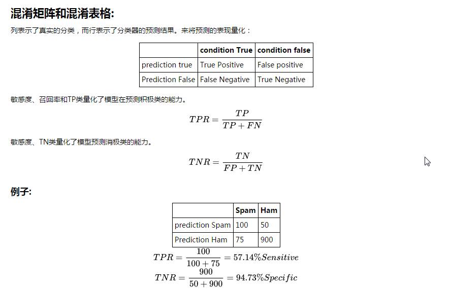
精确率和召回率
计算的数值并不能总是良好的区分好模型与坏模型。它们传达了对模型性能的一些感性认知,而每个数值的有效性与否是由分析者所决定的。准确性的问题在于每次的结果并不一定相同。如果我的分类器预测客户会流失,而实际上他们没有,这不是最好的分类结果,但这个结果是可以被原谅的。然而,如果我的分类器预测客户会留下,因而我就没有发现他们实际上是要流失的客户…那这就是糟糕的分类结果。
我将使用另一个内置的scikit-learn函数来构造混淆矩阵。混淆矩阵是一种将分类器预测结果的可视化的方法,并且仅仅是一个表格,其示出了对于特定类的预测的分布。x轴表示每个观察的真实类别(如果客户流失或不流失),而y轴对应于模型预测的类别(如果我的分类器表示客户会流失或不流失)。
T
N
R
=
900
50
+
900
=
94.73
%
S
p
e
c
i
f
i
c
In [10]:
from sklearn.metrics import confusion_matrix
from sklearn.metrics import precision_score
from sklearn.metrics import recall_scored
ef draw_confusion_matrices(confusion_matricies,class_names):
class_names = class_names.tolist()
for cm in confusion_matrices:
classifier, cm = cm[0], cm[1]
print(cm)
fig = plt.figure()
ax = fig.add_subplot(111)
cax = ax.matshow(cm)
plt.title('Confusion matrix for %s' % classifier)
fig.colorbar(cax)
ax.set_xticklabels([''] + class_names)
ax.set_yticklabels([''] + class_names)
plt.xlabel('Predicted')
plt.ylabel('True')
plt.show()
y = np.array(y)class_names = np.unique(y)confusion_matrices = [
( "Support Vector Machines", confusion_matrix(y,run_cv(X,y,SVC)) ),
( "Random Forest", confusion_matrix(y,run_cv(X,y,RF)) ),
( "K-Nearest-Neighbors", confusion_matrix(y,run_cv(X,y,KNN)) ),
( "Gradient Boosting Classifier", confusion_matrix(y,run_cv(X,y,GBC)) ),
( "Logisitic Regression", confusion_matrix(y,run_cv(X,y,LR)) )]# Pyplot code not included to reduce clutter# from churn_display import draw_confusion_matrices%matplotlib inlinedraw_confusion_matrices(confusion_matrices,class_names)
[[2818   32]
 [ 247  236]]
[[2832   18]
 [ 173  310]]
[[2808   42]
 [ 306  177]]
[[2821   29]
 [ 126  357]]
[[2770   80]
 [ 385   98]]
要注意的是当客户流失时,分类器的预测正确率如何?这种计算方法被成为召回率,并且快速查看图片可以证明迭代决策树和随机森林在这个标准的计算方法判定上是表现最佳的。在召回率上迭代决策树和随机森林中都达到了大约70%,相比于其他的分类方法远远领先。
另一个要注意的问题是当分类器预测出某用户会流失时,该用户究竟是否会流失?这种计算方法叫做精确度。可以发现在这个计算方法中,突出的仍旧是迭代决策树和随机森林。在精确度上都达到了大约90%,支持向量机也达到了88%。knn算法中也稍微滞后,达到了80%。
然而就如准确度、精确度和召回率中随机森林和迭代决策树都优于其他的分类方法,但是并不是在所有的情形中,这两类分类方法都能够优于其他的分类方法。而如果不同的计算方法中返回了不同的优劣排序,那么针对于不同计算方法中所包含的内容和价值,就能够选出最适合的分类方法。
ROC 曲线 & AUC
另一个重要的指标是ROC图。
简而言之,ROC曲线下的面积(AUC)是将查看ROC曲线的评价结果简化为了对于面积大小的判断。 对于二值分类器系统,ROC曲线绘制了真正的TP(sensitivity)与FP(1 - specificity),随着其鉴别阈值是变化的。 在随机方法下AUC为0.5。因此我们可以直观的说分类器应该比随机判断的情况好,因此分类结果的ROC曲线面积越大,就有越好的预期性能。
In [11]:
from sklearn.metrics import roc_curve, auc
from scipy import interp
def plot_roc(X, y, clf_class, **kwargs):
kf = KFold(len(y), n_folds=5, shuffle=True)
y_prob = np.zeros((len(y),2))
mean_tpr = 0.0
mean_fpr = np.linspace(0, 1, 100)
all_tpr = []
for i, (train_index, test_index) in enumerate(kf):
X_train, X_test = X[train_index], X[test_index]
y_train = y[train_index]
clf = clf_class(**kwargs)
clf.fit(X_train,y_train)
# Predict probabilities, not classes
y_prob[test_index] = clf.predict_proba(X_test)
fpr, tpr, thresholds = roc_curve(y[test_index], y_prob
[test_index, 1])
mean_tpr += interp(mean_fpr, fpr, tpr)
mean_tpr[0] = 0.0
roc_auc = auc(fpr, tpr)
plt.plot(fpr, tpr, lw=1, label='ROC fold %d (area = %0.2f)' % (i, roc_auc))
mean_tpr /= len(kf)
mean_tpr[-1] = 1.0
mean_auc = auc(mean_fpr, mean_tpr)
plt.plot(mean_fpr, mean_tpr, 'k--',label='Mean ROC (area = %0.2f)' % mean_auc, lw=2)
plt.plot([0, 1], [0, 1], '--', color=(0.6, 0.6, 0.6), label='Random')
plt.xlim([-0.05, 1.05])
plt.ylim([-0.05, 1.05])
plt.xlabel('False Positive Rate')
plt.ylabel('True Positive Rate')
plt.title('Receiver operating characteristic')
plt.legend(loc="lower right")
plt.show()
print ("Support vector machines:")
plot_roc(X,y,SVC,probability=True)
print ("Random forests:")plot_roc(X,y,RF,n_estimators=18)print ("K-nearest-neighbors:")plot_roc(X,y,KNN)print ("Gradient Boosting Classifier:")plot_roc(X,y,GBC)
Support vector machines:
Random forests:
K-nearest-neighbors:
Gradient Boosting Classifier:
Feature Importance
在了解了我们特定数据集中模型的准确率后,我们应当深入了解是什么特征和行为引发了客户流失。 我们将使用"RandomForestClassifer"构建决策树的集合来预测客户是否会流失。 ·构建的第一步是计算特定要素上的 现在我们了解了我们特定数据集的每一个模型的准确性,让我们深入了解一下什么特征或行为导致客户流失。 在下一节中,我们将使用“RandomForestClassifer”来构建一个决策树的集合来预测客户是否会流失或不会流失。
我们来看看数据集中的十大要素,有助于客户流失:
In [12]:
train_index,test_index = train_test_split(churn_df.index)forest
= RF()forest_fit = forest.fit(X[train_index], y[train_index])forest_predictions = forest_fit.predict(X[test_index])importances = forest_fit.feature_importances_[:10]std = np.std([tree.feature_importances_ for tree in forest.estimators_],
axis=0)indices = np.argsort(importances)[::-1]
# Print the feature ranking
print("Feature ranking:")
for f in range(10):
print("%d. %s (%f)" % (f + 1, features[f], importances[indices[f]]))
# Plot the feature importances of the forest#import pylab as pl
plt.figure()plt.title("Feature importances")plt.bar(range(10), importances[indices], yerr=std[indices], color="r", align="center")plt.xticks(range(10), indices)
plt.xlim([-1, 10])
plt.show()
Feature ranking:
1. Account Length (0.149028)
2. Int'l Plan (0.138706)
3. VMail Plan (0.080912)
4. VMail Message (0.065540)
5. Day Mins (0.052949)
6. Day Calls (0.038687)
7. Day Charge (0.034273)
8. Eve Mins (0.033965)
9. Eve Calls (0.023378)
10. Eve Charge (0.019477)
Thinking in Probabilities
决策往往有利于简单分类的概率。在“明天有20%的机会下雨”和“大约55%的考生通过加利福尼亚酒吧考试”这样的表述中,比只是说“明天不应该下雨”或“你可能会通过”更有效用。流失的概率预测也使我们能够衡量客户的预期价值及其预期的损失。谁想要首先接触客户,每年支付20万美元的80%的流失风险,或每年价值10万的客户,风险为40%? 你应该在每个客户端上花多少钱?
“scikit-learn”使得概率变得容易; 我的三个模型已经将predict_proba()构建到他们的类对象中。这是相同的交叉验证码,只有几行改变。
In [13]:
def run_prob_cv(X, y, clf_class, roc=False, **kwargs):
kf = KFold(len(y), n_folds=5, shuffle=True)
y_prob = np.zeros((len(y),2))
for train_index, test_index in kf:
X_train, X_test = X[train_index], X[test_index]
y_train = y[train_index]
clf = clf_class(**kwargs)
clf.fit(X_train,y_train)
# Predict probabilities, not classes
y_prob[test_index] = clf.predict_proba(X_test)
return y_prob
什么是最好的算法?
确定给出概率而不是类的预测因子有一定的难度。如果我预测明天有20%的可能性会下雨的,比告诉你下雨还是不下雨更好。 所以每次我预测一个事件发生20%的时间,我可以看到这些事件实际发生的频率。 这里我们将使用“pandas”来帮助我比较随机森林对实际结果的预测。
In [14]:
import warningswarnings.filterwarnings('ignore')
# Use 10 estimators so predictions are all multiples of 0.1
pred_prob = run_prob_cv(X, y, RF, n_estimators=10)
pred_churn = pred_prob[:,1]is_churn = y == 1
# Number of times a predicted probability is assigned to an observation
counts = pd.value_counts(pred_churn)counts[:]
Out[14]:
0.0    1774
0.1     719
0.2     240
0.3     127
0.8      77
0.4      70
1.0      70
0.7      69
0.9      66
0.6      61
0.5      60
dtype: int64
In [15]:
from collections import defaultdicttrue_prob = defaultdict(float)# calculate true probabilitiesfor prob in counts.index:
    true_prob[prob] = np.mean(is_churn[pred_churn == prob])true_prob = pd.Series(true_prob)# pandas-fucounts = pd.concat([counts,true_prob], axis=1).reset_index()counts.columns = ['pred_prob', 'count', 'true_prob']counts
Out[15]:
|
pred_prob
|
count
|
true_prob
|
|
0
|
0.0
|
1774
|
0.027621
|
|
1
|
0.1
|
719
|
0.033380
|
|
2
|
0.2
|
240
|
0.054167
|
|
3
|
0.3
|
127
|
0.157480
|
|
4
|
0.4
|
70
|
0.357143
|
|
5
|
0.5
|
60
|
0.600000
|
|
6
|
0.6
|
61
|
0.754098
|
|
7
|
0.7
|
69
|
0.898551
|
|
8
|
0.8
|
77
|
0.948052
|
|
9
|
0.9
|
66
|
0.984848
|
|
10
|
1.0
|
70
|
1.000000
|
我们可以发现随机森林预测了有75个案例有90%的概率会流失,而实际中改组有97%的比例流失了。
校准和鉴别
使用上面的DataFrame我可以绘制一个非常简单的图形,以帮助可视化概率测量。 x轴表示随机森林分配给一组个体的流失概率。 y轴是该组内实际的流失概率,每个点相对于组的大小进行缩放。校准是一个相对简单的测量,可以总结如下:预测发生的事件60%的时间应该发生在60%的时间。对于所有个人,我预测流失风险在30%至40%之间,该组的真正流失率应为35%左右。对于上面的图表,想到这一点,我对红线的预测有多接近?
歧视措施_我的预测远离绿线?_为什么这么重要?
那么,如果我们为每个人分配15%的流失概率,我们将会因为平均值而接近完美的校准,但是我将缺乏真正的洞察力。如果鉴别能够隔离更远离基础组的组,它给予一个更好的分数的模型
公式来自于 Yang, Yates, and Smith (1991)
In [16]:
from __future__ import division
import numpy as np
def calibration(prob,outcome,n_bins=10):
"""Calibration measurement for a set of predictions.
When predicting events at a given probability, how far is frequency
of positive outcomes from that probability?
NOTE: Lower scores are better
prob: array_like, float
Probability estimates for a set of events
outcome: array_like, bool
If event predicted occurred n_bins: int
Number of judgement categories to prefrom calculation over.
Prediction are binned based on probability, since "descrete"
probabilities aren't required. """
prob = np.array(prob)
outcome = np.array(outcome)
c = 0.0
# Construct bins
judgement_bins = np.arange(n_bins + 1) / n_bins
# Which bin is each prediction in?
bin_num = np.digitize(prob,judgement_bins)
for j_bin in np.unique(bin_num):
# Is event in bin
in_bin = bin_num == j_bin
# Predicted probability taken as average of preds in bin
predicted_prob = np.mean(prob[in_bin])
# How often did events in this bin actually happen?
true_bin_prob = np.mean(outcome[in_bin])
# Squared distance between predicted and true times num of obs
c += np.sum(in_bin) * ((predicted_prob - true_bin_prob) ** 2)
return c / len(prob)def discrimination(prob,outcome,n_bins=10):
"""Discrimination measurement for a set of predictions. For each judgement category, how far from the base probability is the true frequency of that bin? NOTE: High scores are better prob: array_like, float Probability estimates for a set of events outcome: array_like, bool If event predicted occurred n_bins: int Number of judgement categories to prefrom calculation over. Prediction are binned based on probability, since "descrete" probabilities aren't required. """
prob = np.array(prob)
outcome = np.array(outcome)
d
= 0.0
# Base frequency of outcomes
base_prob = np.mean(outcome)
# Construct bins
judgement_bins = np.arange(n_bins + 1) / n_bins
# Which bin is each prediction in?
bin_num = np.digitize(prob,judgement_bins)
for j_bin in np.unique(bin_num):
in_bin = bin_num == j_bin
true_bin_prob = np.mean(outcome[in_bin])
# Squared distance between true and base times num of obs
d += np.sum(in_bin) * ((true_bin_prob - base_prob) ** 2)
return d / len(prob)
In [17]:
from sklearn.metrics import roc_curve, auc
from scipy import interp
from __future__ import division
from operator import *
      def print_measurements(pred_prob):
    churn_prob, is_churn = pred_prob[:,1], y == 1
    print (("  %-20s %.4f" )% ("Calibration Error", calibration(churn_prob, is_churn)))
    print (("  %-20s %.4f") % ("Discrimination", discrimination(churn_prob,is_churn)))

    print ("Note -- Lower calibration is better, higher discrimination is better")
print ("Support vector machines:")
print_measurements(run_prob_cv(X,y,SVC,probability=True))
print ("Random forests:")print_measurements(run_prob_cv(X,y,RF,n_estimators=18))
print ("K-nearest-neighbors:")print_measurements(run_prob_cv(X,y,KNN))
print ("Gradient Boosting Classifier:")print_measurements(run_prob_cv(X,y,GBC))
print ("Random Forest:")print_measurements(run_prob_cv(X,y,RF))
Support vector machines:
  Calibration Error    0.0010
  Discrimination       0.0676
Note -- Lower calibration is better, higher discrimination is better
Random forests:
  Calibration Error    0.0056
  Discrimination       0.0822
Note -- Lower calibration is better, higher discrimination is better
K-nearest-neighbors:
  Calibration Error    0.0031
  Discrimination       0.0460
Note -- Lower calibration is better, higher discrimination is better
Gradient Boosting Classifier:
  Calibration Error    0.0018
  Discrimination       0.0833
Note -- Lower calibration is better, higher discrimination is better
Random Forest:
  Calibration Error    0.0059
  Discrimination       0.0818
Note -- Lower calibration is better, higher discrimination is better
与之前的分类比较不同,随机森林在这里并不明显。 虽然它有利于区分高概率和低概率流失事件,但是在为这些事件分配准确的概率估计时遇到困难。 例如,随机森林预测具有30%流失率的组实际上的真正流失率为14%。
Credits: Forked from
growth-workshop
by
aprial
, as featured on the
yhat blog
推荐阅读:
40行代码的人脸识别实践
如何优雅的使用Python
给Python初学者的一些技巧
干货 : 写给喜欢数据分析的初学者
数据科学的完整学习路径
看看 40 岁“老”程序员的反思


