To round out the week, I thought I’d take a selection of fun papers from the ‘More papers from 2016’ section of
top 100 awesome deep learning papers
list.
The texture networks paper we’ve covered before, so the link in the above list is to The Morning Paper write-up (but I felt like it belonged in this group nevertheless).
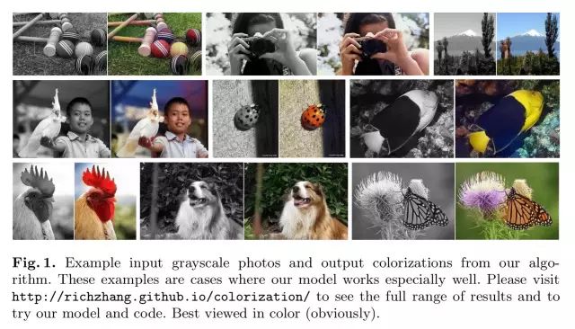
Colorful image colorization
Given a grayscale photograph as input, this paper attacks the problem of hallucinating a
plausible
color version of the photograph.
How is this possible? Well, we’ve seen that networks can learn what various parts of the image represent. If you see enough images you can learn that grass is (usually) green, the sky is (sometimes!) blue, and ladybirds are red. The network doesn’t have to recover the actual ground truth colour, just a plausible colouring.
Therefore, our task becomes much more achievable: to model enough of the statistical dependencies between the semantics and the textures of grayscale images and their color versions in order to produce visually compelling results.
Results like this:
Training data for the colourisation task is plentiful – pretty much any colour photo will do. The tricky part is finding a good loss function – as we’ll see soon, many loss functions produce images that look desaturated, whereas we want vibrant realistic images.
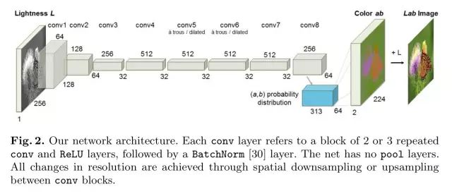
The network is based on image data using the
CIE
Lab
colourspace
. Grayscale images have only the lightness, L, channel, and the goal is to predict the
a
(green-red) and
b
(blue-yellow) colour channels. The overall network architecture should look familiar by now, indeed so familiar that supplementary details are pushed to an
accompanying website
.
(That website page is well worth checking out by the way, it even includes a link to a demo site on Algorithmia where you can
try the system out for yourself on your own images
).
Colour prediction is inherently
multi-modal
, objects can take on several plausible colourings. Apples for example may be red, green, or yellow, but are unlikely to be blue or orange. To model this, the prediction is a distribution of possible colours for each pixel. A typical objective function might use e.g. Euclidean loss between predicted and ground truth colours.
However, this loss is not robust to the inherent ambiguity and multimodal nature of the colorization problem. If an object can take on a set of distinct
ab
values, the optimal solution to the Euclidean loss will be the mean of the set. In color prediction, this averaging effect favors grayish, desaturated results. Additionally, if the set of plausible colorizations is non-convex, the solution will in fact be out of the set, giving implausible results.
What can we do instead? The
ab
output space is divided into bins with grid size 10, and the top
Q
= 313 in-gamut (within the range of colours we want to use) are kept:

The network learns a mapping to a probability distribution over these Q colours (a Q-dimensional vector). The ground truth colouring is also translated into a Q-dimensional vector, and the two are compared using a multinomial cross entropy loss. Notably this includes a weighting term to rebalance loss based on colour-class rarity.
The distribution of ab values in natural images is strongly biased towards values with low ab values, due to the appearance of backgrounds such as clouds, pavement, dirt, and walls. Figure 3(b) [below] shows the empirical distribution of pixels in ab space, gathered from 1.3M training images in ImageNet. Observethat the number of pixels in natural images at desaturated values are orders of magnitude higher than for saturated values. Without accounting for this, the loss function is dominated by desaturated
ab
values.

The final predicted distribution then needs to be mapped to a point estimated in
ab
space. Taking the
mode
of the predicted distribution leads to vibrant but sometimes spatially inconsistent results (see RH column below). Taking the
mean
brings back another form of the desaturation problem (see LH column below).


