
本文将以反应时数据分析为例详细介绍
如何使用R语言进行
混合效应模型
(
Mixed-Effects Models
)
分析
(Freeman, Heathcote, Chalmers & Hockley, 2010)
。这是对曾发布于
“荷兰心理统计联盟”的
使用R语言进行混合线性模型(mixed linear model) 分析代码及详解
和“表哥有话讲”的
基于R的混合线性模型的实现
两篇文章的进一步扩充。
混合效应模型
(Mixed-Effects Models)
,
是指同时包含固定效应
(fixed effects)
及随机效应
(random effects)
的模型。其
在不同领域有一些近义词,如多层线性模型
(Hierarchical Linear Model)
、线性混合模型
(Linear Mixed Model)
等。
本次分析中所用到的反应时原始数据来自
Freeman
等人的研究
(Freeman et al., 2010)
,
Freeman
等人采用
2(task:lexical decision task vs. naming task)×2(neighborhood density:low vs. high)×2(stimulus frequency)×2(stimulus:word vs. nonword)
的四因素混合实验设计(如图1所示),其中
task
为被试间变量,其余均为被试内变量。研究共招募了
45
名被试(词汇判断任务
25
名,命名任务
20
人)对
300
个单词
(words)
和
300
个非词
(nonwords)
的词汇判断反应时
(lexical decision latencies)
以及命名反应时
(word naming latencies)
。
首先导入原始数据和所有分析所需的统计包,见下图。注意我们剔除掉了原始数据当中所有错误反应的试次。
library("afex") # needed for mixed() and attaches lme4 automatically.library("emmeans") # emmeans is needed for follow-up tests (and not anymore loaded automatically).library("multcomp") # for advanced control for multiple testing/Type 1 errors.library("dplyr") # for working with data frameslibrary("tidyr") # for transforming data frames from wide to long and the other way round.library("lattice") # for plotslibrary("latticeExtra") # for combining lattice plots, etc.
lattice.options(default.theme = standard.theme(color = FALSE)) # black and whitelattice.options(default.args = list(as.table = TRUE)) # better ordering
data("fhch2010") # load fhch # remove errorsstr(fhch2010) # structure of the data## 'data.frame':    13222 obs. of  10 variables:##  $ id       : Factor w/ 45 levels "N1","N12","N13",..: 1 1 1 1 1 1 1 1 1 1 ...##  $ task     : Factor w/ 2 levels "naming","lexdec": 1 1 1 1 1 1 1 1 1 1 ...##  $ stimulus : Factor w/ 2 levels "word","nonword": 1 1 1 2 2 1 2 2 1 2 ...##  $ density  : Factor w/ 2 levels "low","high": 2 1 1 2 1 2 1 1 1 1 ...##  $ frequency: Factor w/ 2 levels "low","high": 1 2 2 2 2 2 1 2 1 2 ...##  $ length   : Factor w/ 3 levels "4","5","6": 3 3 2 2 1 1 3 2 1 3 ...##  $ item     : Factor w/ 600 levels "abide","acts",..: 363 121 202 525 580 135 42 368 227 141 ...##  $ rt       : num  1.091 0.876 0.71 1.21 0.843 ...##  $ log_rt   : num  0.0871 -0.1324 -0.3425 0.1906 -0.1708 ...##  $ correct  : logi  TRUE TRUE TRUE TRUE TRUE TRUE .
然后,检查一下每种条件下的被试数量和每位被试所接受的实验刺激数量。这个需要借助
‘dplyr’
包里面的功能实现。
#fhch2010 %>% group_by(id) %>% summarise(task = n_distinct(task)) %>% as.data.frame() %>% {.$task == 1} %>% all()##fhch2010 %>% group_by(id) %>% summarise(task = first(task)) %>% ungroup() %>% group_by(task) %>% summarise(n = n())######fhch2010 %>% group_by(id, stimulus) %>% summarise(items = n_distinct(item)) %>% ungroup() %>% group_by(stimulus) %>% summarise(min = min(items), max = max(items), mean = mean(items))#####
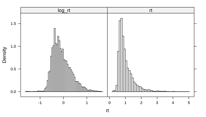
本次数据分析的因变量是反应时,通常来说,反应时都是呈正偏态分布的,因此,我们对其进行了
log
转换来使其更“正态”一些。下面的代码分别绘制了
log_rt
和
rt
的分布,从图上看,采用log转换确实让分布看起来更“正态”了一些。
如果原始数据呈正态分布,那直接使用原始数据进行分析。当原始数据非正态分布时,或者用
density
来看不是线性分布,需要进行
log
转换,以符合基本假设。
在很多时候,两种都可以分析一下,如果没有特别大差别,详细注明本次数据结果是原始数据,还是
log
后数据。因为不同分析方法,直接导致后续不同方面
译者注:但需要注意的是,跟传统统计分析
(
如
ANOVA)
数据分布需要符合正态分布的假设以外,
mixed-effects models
并没有数据分布一定要正态这一前提条件,相反,
mixed-effects models
的一个优点就在于它能
handle
不同分布的数据。因此,笔者这里内心存疑—我们真的需要对反应时数据进行
log
转换吗?
fhch_long % gather("rt_type", "rt", rt, log_rt)histogram(~rt|rt_type, fhch_long, breaks = "Scott", type = "density", scale = list(x = list(relation = "free")))
重新回顾一下我们的变量:被试间变量
task (lexical decision task vs. naming task)
;被试内变量
stimulus (word vs. nonword), density (low vs. high), frequency (low vs. high)。
在进行正式分析之前,可以图示化我们的数据,看看数据结果跟我们内心的预期是否符合。由于所有的数据都嵌套
(nested data structure)
在被试水平
(participant-level)
和刺激水平
(item-level)
上,下面我们分别来查看两种水平上的数据结果趋势。
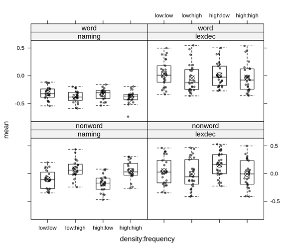
被试水平
(participant-level)
上的数据趋势,注意
 表示每组的均值。
agg_p % group_by(id, task, stimulus, density, frequency) %>% summarise(mean = mean(log_rt)) %>% ungroup()xyplot(mean ~ density:frequency|task+stimulus, agg_p, jitter.x = TRUE, pch = 20, alpha = 0.5, panel = function(x, y, ...) { panel.xyplot(x, y, ...) tmp list(x), mean) panel.points(tmp$x, tmp$y, pch = 13, cex =1.5) }) + bwplot(mean ~ density:frequency|task+stimulus, agg_p, pch="|", do.out = FALSE)
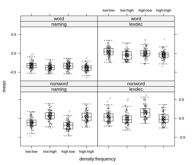
刺激水平
(
item-level
)
上的数据趋势,注意
表示每组的均值。
agg_i % group_by(item, task, stimulus, density, frequency) %>% summarise(mean = mean(log_rt)) %>% ungroup()xyplot(mean ~ density:frequency|task+stimulus, agg_i, jitter.x = TRUE, pch = 20, alpha = 0.2, panel = function(x, y, ...) { panel.xyplot(x, y, ...) tmp list(x), mean) panel.points(tmp$x, tmp$y, pch = 13, cex =1.5) }) + bwplot(mean ~ density:frequency|task+stimulus, agg_i, pch="|", do.out = FALSE)
结合上面的绘图我们初步可以得出以下结果:
①对于命名任务
(naming task)
来说,非词汇
(nonword)
反应时
>
词汇
(word)
反应时。
②就词汇
(word)
反应时而言,被试在词汇判断任务
(lexical decision task)
中的整体反应>在命名任务
(naming task)
中的整体反应。
③在命名任务
(naming task)
中,
frequency
对非词汇
(nonword)
反应时的主效应显著。
④就词汇
(word)
反应时而言,无论是命名任务
(naming task)
还是词汇判断任务
(lexical decision task)
,似乎低频词汇所需要的反应时更长。
⑤从图上看,
density
在四种情况下的主效应均不显著。
1
首先,从理念上来讲,
mixed-effects models
的建立分两种取向:
第一种
是
"maximal model approach"(Barr, Levy, Scheepers, & Tily, 2013)
,即一开始就放入所有能放入的
random intercepts, random slopes
和
random correlations。
如果模型有问题,再进行删减。
第二种
则是一开始先跑一个比较简单一点的模型(如:只放
random intercepts,
不放
random slopes and randomcorrelations)
,然后再次基础之上慢慢添加变量。本例将采取的是
"maximal model approach"。
译者个人是倾向于
‘maximal model approach’
的。既然
mixed-effects models
最大的优势在于能同时考察
fixed effects
并控制
random effects,
那么理论上一开始我们就应该在模型中控制所有能控制的
random effects
才对。如果采用
"simple model approach",
可以想象一开始模型不会出现什么大的问题
(
如
: convergence problem, singularityfit)
,然后再慢慢添加变量,直到模型出现问题就停止,这种做法本质上跟
p-hacking
没有什么区别,不是对待科学应有的态度。
1
第二步,我们来确定
random intercepts
和
random slopes。
由于所有的数据都嵌套
(nested data structure)
在被试水平
(participant-level)
和刺激水平
(item-level)
上,所以我们的
random intercepts
也就出来了,就是每位被试的
id
以及
item
。
接下来是
random slopes。
在被试水平
(participant-level)
上共有三个变量可以纳入作为
random slopes: stimulus,density, frequency;
在刺激水平
(item-level)
上则只有
task
这一个变量可以作为
random slope。
1
第三步,需要注意有些时候跑模型会遇到
convergence problem
或者
singularity fit。
这个时候你的模型可能没有问题,但是
R
却无法确定此时此刻你的模型是否是最优解。
遇到这种情况,一种解决办法是稍微简化一下原有的
"maximal model"
,通常的做法是去掉
random correlations,
只保留
random intercepts andrandom slopes。
照着这个思路,本例中我们一共会跑如下四个模型:
(1) 保留所有的
random intercepts, randomslopes and random correlations—see model 1 in Table 1。
(2) 只去掉刺激水平
(item-level)
上的
random correlation—see model 2 in Table 1。
(3) 只去掉被试水平
(participant-level)
上的
random correlation—see model 3 in Table 1。
(4) 既去掉被试水平
(participant-level)
上又去掉刺激水平
(item-level)
上的
random correlations—see model 4 in Table 1。
Mixed-Effects Models and Mixed Syntax in R
|
|
|
|
|
afex::mixed(task*stimulus*density*frequency +(stimulus*density*frequency | id) + (task | item))
|
|
|
afex::mixed(log_rt ~ task*stimulus*density*frequency + (stimulus*density*frequency | id) +(task || item))
|
|
|
afex::mixed(log_rt ~ task*stimulus*density*frequency + (stimulus*density*frequency || id) +(task | item))
|
|
|
afex::mixed(log_rt ~ task*stimulus*density*frequency + (stimulus*density*frequency || id) +(task || item))
|
Note. (A) We ran all mixed-effects models using the ‘mixed’ function from the‘afex’ package in R. (B) In R the effect of A * B = the main effect of A + themain effect of B + the interaction between A and B. (C) The ‘||’ means removingrandom correlations.
1
第四步,计算
p-values
。一般有三种方法:
LRT(=LikelihoodRatio-Tests),
KR (= Kenward-Roger) F test,
the ‘Satterthwaite’ approximation。
前人研究表明
(Luke, 2017)
,这三种方法各有利弊,但相对来说目前效果最好的是
KR F test,
最不推荐
LRT
。
在本例中我们将采用
‘Scatterthwaite’ approximation
和
LRT
。还有一种策略就是这三种方法都试一遍,如果能得到相同的分析结果,侧面也说明了结果的可靠性和稳健性。
#----------------Satterthwaite Results------------m1s id)+               (task|item), fhch, method = "S",              control = lmerControl(optCtrl = list(maxfun = 1e6)))m2s id)+               (task||item), fhch, method = "S",              control = lmerControl(optCtrl = list(maxfun = 1e6)), expand_re = TRUE)m3s id)+               (task|item), fhch, method = "S",              control = lmerControl(optCtrl = list(maxfun = 1e6)), expand_re = TRUE)m4s id)+               (task||item), fhch, method = "S",              control = lmerControl(optCtrl = list(maxfun = 1e6)), expand_re = TRUE)load(system.file("extdata/", "freeman_models.rda", package = "afex"))
m1s m2sm3sm4s
以下分别是四个模型的结果,注意如果我们遇到了
"
convergence problem"
,在模型结果部分会出现
Warnings。
> Model 1
##########################
> Model 2
##########################
> Model 3
> Model 4
总结一下以上的结果。
首先,
Model 1
和
Model 2
都出现了
convergence problem,
而
Model 3
和
Model 4
则没有。请注意
convergence problem
并不是说模型本身出现了问题,而是
R
并不确定当前的模型是否是拟合数据的最优解。
其次,除了
Model 1
无法提供
p-values
以外,
Model 2, Model 3
和
Model 4
都得出了同样的分析结果—几乎完全相同的
Effect
值,
df
值,
F
值以及
p-values
。这说明我们之前遇到的
convergence problem
是一个
false positive
,我们可以不用再担心它了。
我们得到了
2
个显著的主效应:
main effects for taskand stimulus。
四个显著的二阶交互作用
: ‘task: stimulus’, ‘task : density’, ‘task : frequency’, and ‘stimulus : frequency’
。三个显著的三阶交互作用:
‘task: stimulus : density’, ‘task : stimulus : frequency’, and ‘task : density :frequency’。
一个边缘显著的三阶交互作用:
stimulus : density :frequency。
一个显著的四阶交互作用
: task : stimulus : density : frequency。
使用
LRT Methods
跑模型得出了和上述一致的分析结果,这让我们对分析结果有了更充足的信心。具体见
R
代码。
#-------------------------------- LRT Results ------------------------------m1lrt id)+                 (task|item), fhch, method = "LRT",                control = lmerControl(optCtrl = list(maxfun = 1e6)))m2lrt id)+                 (task||item), fhch, method = "LRT",                control = lmerControl(optCtrl = list(maxfun = 1e6)), expand_re = TRUE)m3lrt id)+                 (task|item), fhch, method = "LRT",                control = lmerControl(optCtrl = list(maxfun = 1e6)), expand_re = TRUE)m4lrt id)+                 (task||item), fhch, method = "LRT",                control = lmerControl(optCtrl = list(maxfun = 1e6)), expand_re = TRUE)

res_lrt 1]], "  " = " ",                  nice_lrt[[4]][,-(1:2)])colnames(res_lrt)[c(3,4,6,7)]   rep(c("m1_", "m4_"), each =2), colnames(res_lrt)[c(3,4)])res_lrt
nice_lrt[[2]]
我们用
R
当中的
‘emmeans’ package
来进行事后比较。本例中将着重分析两个交互作用:
‘task : stimulus :frequency’ interaction and ‘task : stimulus :density : frequency’ interaction。


