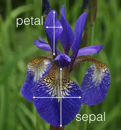
iris数据集是由三种鸢尾花,各50组数据构成的数据集。每个样本包含4个特征,分别为萼片(sepals)的长和宽、花瓣(petals)的长和宽。
In [36]:
from sklearn.datasets import
load_irisiris = load_iris()
type(iris)
Out[36]:
sklearn.datasets.base.Bunch
In [37]:
print(iris.feature_names)
print(iris.target_names)
['sepal length (cm)', 'sepal width (cm)', 'petal length (cm)', 'petal width (cm)']
['setosa' 'versicolor' 'virginica']
在scikit-learn中对数据有如下要求:
特征和标签要用分开的对象存储
特征和标签要是数字
特征和标签都要使用numpy的array来存储
In [38]:
print(type(iris.data))
print(type(iris.target))
In [39]:
print(iris.data.shape)
print(iris.target.shape)
(150, 4)
(150,)
In [40]:
# store features matrix in "X"
X = iris.data
# store response vector in "y"
y = iris.target
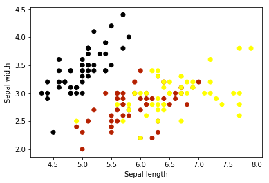
绘制iris的2d图
In [41]:
%matplotlib inline
import matplotlib.pyplot as plt
X_sepal = X[:, :2]
plt.scatter(X_sepal[:, 0], X_sepal[:, 1], c=y, cmap=plt.cm.gnuplot)
plt.xlabel('Sepal length')plt.ylabel('Sepal width')
Out[41]:
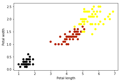
In [42]:
X_petal = X[:, 2:4]
plt.scatter(X_petal[:, 0], X_petal[:, 1], c=y, cmap=plt.cm.gnuplot)
plt.xlabel('Petal length')plt.ylabel('Petal width')
Out[42]:
使用K近邻进行分类
KNN分类的基本步骤:
选择K的值
在训练数据集中搜索K个距离最近的观测值
使用最多的那个标签作为未知数据的预测
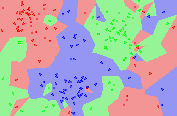
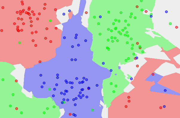
下面给出KNN的演示图例, 分别是训练数据、K=1时的KNN分类图、K=5时的KNN分类图
scikit-learn进行模型匹配的4个一般步骤
第一步:载入你要使用的模型类
In [43]:
from sklearn.neighbors import KNeighborsClassifier
第二步:实例化分类器
In [44]:
# looking for the one nearest neighbor
knn = KNeighborsClassifier(n_neighbors=1)
In [45]:
print(knn)
KNeighborsClassifier(algorithm='auto', leaf_size=30, metric='minkowski',
           metric_params=None, n_jobs=1, n_neighbors=1, p=2,
           weights='uniform')
第三步:用数据来拟合模型(进行模型的训练)
In [46]:
knn.fit(X, y)
Out[46]:
KNeighborsClassifier(algorithm='auto', leaf_size=30, metric='minkowski',
           metric_params=None, n_jobs=1, n_neighbors=1, p=2,
           weights='uniform')
第四步:对新的观测值进行预测
In [47]:
knn.predict([3, 5, 4, 2])
/opt/conda/lib/python3.5/site-packages/sklearn/utils/validation.py:395: DeprecationWarning: Passing 1d arrays as data is deprecated in 0.17 and will raise ValueError in 0.19. Reshape your data either using X.reshape(-1, 1) if your data has a single feature or X.reshape(1, -1) if it contains a single sample.
  DeprecationWarning)
Out[47]:
array([2])
In [48]:
X_new = [[3, 5, 4, 2], [5, 4, 3, 2]]knn.predict(X_new)
Out[48]:
array([2, 1])
使用不同的K值
In [49]:
knn5 = KNeighborsClassifier(n_neighbors=5)
knn5.fit(X, y)
knn5.predict(X_new)
Out[49]:
array([1, 1])
依照同样的流程,使用不同的分类模型
In [50]:
# import the class
from sklearn.linear_model import LogisticRegression
# instantiate the model (using the default parameters)
logreg = LogisticRegression()
# fit the model with data
logreg.fit(X, y)
# predict the response for new observations
logreg.predict(X_new)
Out[50]:
array([2, 0])
内容概要
这一节我们介绍以下几个内容:
我们该怎样选择模型用于监督学习任务?
我们该如何选择调整得到最好的模型参数?
我们该如何对测试数据进行预测估计?
使用整个数据集进行训练和测试
In [51]:
from sklearn.datasets import
load_irisiris = load_iris()
# create X(features) and y(response)
X = iris.datay = iris.target
Logistic regression
In [52]:
from sklearn.linear_model import LogisticRegression
logreg = LogisticRegression()
logreg.fit(X, y)
y_pred = logreg.predict(X)
print(("predicted response:\n",y_pred))
('predicted response:\n', array([0, 0, 0, 0, 0, 0, 0, 0, 0, 0, 0, 0, 0, 0, 0, 0, 0, 0, 0, 0, 0, 0, 0,
       0, 0, 0, 0, 0, 0, 0, 0, 0, 0, 0, 0, 0, 0, 0, 0, 0, 0, 0, 0, 0, 0, 0,
       0, 0, 0, 0, 1, 1, 1, 1, 1, 1, 1, 1, 1, 1, 1, 1, 1, 1, 1, 1, 2, 1, 1,
       1, 2, 1, 1, 1, 1, 1, 1, 1, 1, 1, 1, 1, 1, 2, 2, 2, 1, 1, 1, 1, 1, 1,
       1, 1, 1, 1, 1, 1, 1, 1, 2, 2, 2, 2, 2, 2, 2, 2, 2, 2, 2, 2, 2, 2, 2,
       2, 2, 2, 2, 2, 2, 2, 2, 2, 2, 2, 2, 2, 2, 1, 2, 2, 2, 2, 2, 2, 2, 2,
       2, 2, 2, 2, 2, 2, 2, 2, 2, 2, 2, 2]))
In [53]:
len(y_pred)
Out[53]:
150
分类准确率
现在我们需要使用一种度量方式来评价我们的模型的运行情况,我们使用正确预测的比例来作为评估的度量(evaluation metric)。
In [54]:
from sklearn import metrics
print((metrics.accuracy_score(y, y_pred)))
0.96
以上说明对于训练的数据,我们有96%的数据预测正确。这里我们使用相同的数据来训练和预测,使用的度量称其为训练准确度。
KNN(K=5)
In [55]:
from sklearn.neighbors import KNeighborsClassifier
knn5 = KNeighborsClassifier(n_neighbors=5)
knn5.fit(X, y)
y_pred = knn5.predict(X)
print((metrics.accuracy_score(y, y_pred)))
0.966666666667
KNN(K=1)
In [56]:
knn1 = KNeighborsClassifier(n_neighbors=1)
knn1.fit(X, y)
y_pred = knn1.predict(X)
print((metrics.accuracy_score(y, y_pred)))
1.0
上面我们得到了训练准确度为100%的模型,貌似得到了最好的模型和参数。但我们回想一下KNN算法的原理,KNN算法寻找训练数据中的K个最近的数据,它使用指向最多的那个类别来作为预测的输出。
这下我们就明白了为什么当K=1的时候KNN算法的训练准确度为1,KNN会查找在训练数据集中的最近的观测,训练得到的模型会在相同的数据集中找到相同的观测。换句话说,KNN算法已经记住了训练数据集,因为我们使用同样的数据作为测试的数据。
小结
我们要明确训练模型的目的是得到对于未来的观测数据的良好的预测性能,如果我们只是试图最大化训练的准确率,很有可能得到的是针对训练数据的过于复杂的模型,这种模型不具有很好的泛化能力,也就是说对于未知数据的预测得不到很好的性能。
构建没有必要的过于复杂的模型被称作过拟合。这样的模型过分地拟合噪声数据,胜过去拟合信号数据。在KNN模型中,小K值的模型会生成复杂度很高的模型,因为它跟随数据中的噪声。
下面这个是过拟合的一幅图像: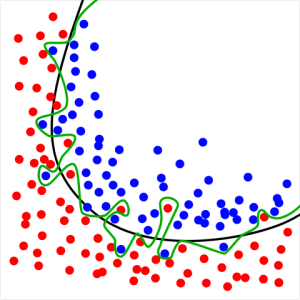 这里绿色的分割线努力去学习噪声的规律,而不像黑色的分割线去学习数据信号的规律,这样对比之下,黑色的线的泛化能力应该更好。
分别设置训练集和测试集
将数据集分成两部分:训练集和测试集
使用训练集对模型进行训练
使用测试集进行模型的测试并评估性能如何
In [57]:
print((X.shape))print((y.shape))
# 第一步:将X和y分割成训练和测试集
from sklearn.cross_validation import train_test_split
X_train, X_test, y_train, y_test = train_test_split(X, y, test_size=0.4, random_state=4)
# 这里的random_state参数根据给定的给定的整数,得到伪随机生成器的随机采样
(150, 4)
(150,)
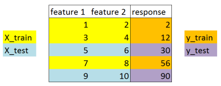 上面这个图告诉我们train_test_split函数的功能,将一个数据集分成两部分。这样使用不同的数据集对模型进行分别的训练和测试,得到的测试准确率能够更好的估计模型对于未知数据的预测效果。
这里测试数据的大小没有统一的标准,一般选择数据集的20%-40%作为测试数据。
In [58]:
print((X_train.shape))
print((X_test.shape))
(90, 4)
(60, 4)
In [59]:
print((y_train.shape))
print((y_test.shape))
(90,)
(60,)
In [60]:
# 第二步:使用训练数据训练模型
logreg = LogisticRegression()
logreg.fit(X_train, y_train)
Out[60]:
LogisticRegression(C=1.0, class_weight=None, dual=False, fit_intercept=True,
          intercept_scaling=1, max_iter=100, multi_class='ovr', n_jobs=1,
          penalty='l2', random_state=None, solver='liblinear', tol=0.0001,
          verbose=0, warm_start=False)
In [61]:
# 第三步: 针对测试数据进行预测,并得到测试准确率
y_pred = logreg.predict(X_test)
print((metrics.accuracy_score(y_test, y_pred)))
# 可以尝试一下,对于上面不同数据集分割,得到的测试准确率不同
0.95
使用KNN算法
In [62]:
# K=5
knn5 = KNeighborsClassifier(n_neighbors=5)
knn5.fit(X_train, y_train)
y_pred = knn5.predict(X_test)

print((metrics.accuracy_score(y_test, y_pred)))
0.966666666667
In [63]:
# K=1
knn1 = KNeighborsClassifier(n_neighbors=1)
knn1.fit(X_train, y_train)
y_pred = knn1.predict(X_test)
print((metrics.accuracy_score(y_test, y_pred)))
0.95
我们能找到一个比较好的K值吗?
In [64]:
# 测试从K=1到K=25,记录测试准确率
k_range = list(range(1, 26))
test_accuracy = []
for k in k_range:
    knn = KNeighborsClassifier(n_neighbors=k)
    knn.fit(X_train, y_train)
    y_pred = knn.predict(X_test)
    test_accuracy.append(metrics.accuracy_score(y_test, y_pred))
In [65]:
%matplotlib inline
import matplotlib.pyplot as plt
plt.plot(k_range, test_accuracy)
plt.xlabel("Value of K for KNN")
plt.ylabel("Testing Accuracy")
Out[65]:
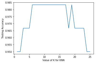
模型参数的选择
在这里,我们选择K的值为11,因为在K=11时,有较高的测试准确率。
In [66]:
# 这里我们对未知数据进行预测
knn11 = KNeighborsClassifier(n_neighbors=11)
knn11.fit(X, y)
knn11.predict([3, 5, 4, 2])
/opt/conda/lib/python3.5/site-packages/sklearn/utils/validation.py:395: DeprecationWarning: Passing 1d arrays as data is deprecated in 0.17 and will raise ValueError in 0.19. Reshape your data either using X.reshape(-1, 1) if your data has a single feature or X.reshape(1, -1) if it contains a single sample.
  DeprecationWarning)
Out[66]:
array([1])
小结
这种分割训练和测试数据集的模型评估流程的缺点是:这种方式会导致待预测数据(out-of-sample)估计准确率的方差过高。因为这种方式过于依赖训练数据和测试数据在数据集中的选择方式。一种克服这种的缺点的模型评估流程称为K折交叉验证,这种方法通过多次反复分割训练、测试集,对结果进行平均。
K折交叉检验
K折将数据集分成K个部分,其中K-1组数据作为构建预测函数的训练之用,剩余的一组数据作为测试之用。
In [67]:
from sklearn.cross_validation import KFold
import numpy as np
def cv_estimate(k, kfold=5):
    cv = KFold(n = X.shape[0], n_folds=kfold)
    clf = KNeighborsClassifier(n_neighbors=k)
    score = 0
    for train, test in cv:
        clf.fit(X[train], y[train])
        score += clf.score(X[test], y[test])
        #print clf.score(X[test], y[test])
    score /= kfold
    return score
In [68]:
# 测试从K=1到K=25,记录测试准确率
k_range = list(range(1, 26))
test_accuracy = []
for k in k_range:
    test_accuracy.append(cv_estimate(k, 5))
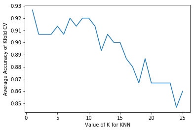
In [69]:
print(test_accuracy)
[0.92666666666666653, 0.90666666666666662, 0.90666666666666662, 0.90666666666666662, 0.91333333333333333, 0.90666666666666662, 0.92000000000000015, 0.91333333333333333, 0.92000000000000015, 0.92000000000000015, 0.91333333333333344, 0.89333333333333331, 0.90666666666666662, 0.90000000000000002, 0.90000000000000002, 0.88666666666666671, 0.88000000000000012, 0.86666666666666659, 0.88666666666666671, 0.86666666666666681, 0.86666666666666681, 0.86666666666666681, 0.86666666666666681, 0.84666666666666668, 0.85999999999999999]
In [70]:
plt.plot(k_range, test_accuracy)
plt.xlabel("Value of K for KNN")
plt.ylabel("Average Accuracy of Kfold CV")
Out[70]: