(点击
上方蓝字
,快速关注我们)
来源:伯乐在线专栏作者 - iPytLab
如有好文章投稿,请点击 → 这里了解详情
前言
最近在写文章需要绘制一些一维的能量曲线(energy profile)和抽象的二维和三维的网格来表示晶体用来描述自己的算法,于是自己在之前的脚本的基础上进行了整改写成了只提供接口的Python库。
基本思想就是封装了matplotlib中相关接口,方便快速搭建和定制自己的能量曲线和网格结构, 代码托管在GitHub上并上传至PyPI。对于研究晶体材料的同学如果想通过python来绘制简单的晶格图像可以参考一下。
GitHub地址: https://github.com/PytLab/catplot/
PyPI地址: https://pypi.python.org/pypi/catplot/
正文
首先还是介绍一下这个程序的用途,目前主要是提供三个主要的模块来绘制三方面的内容:
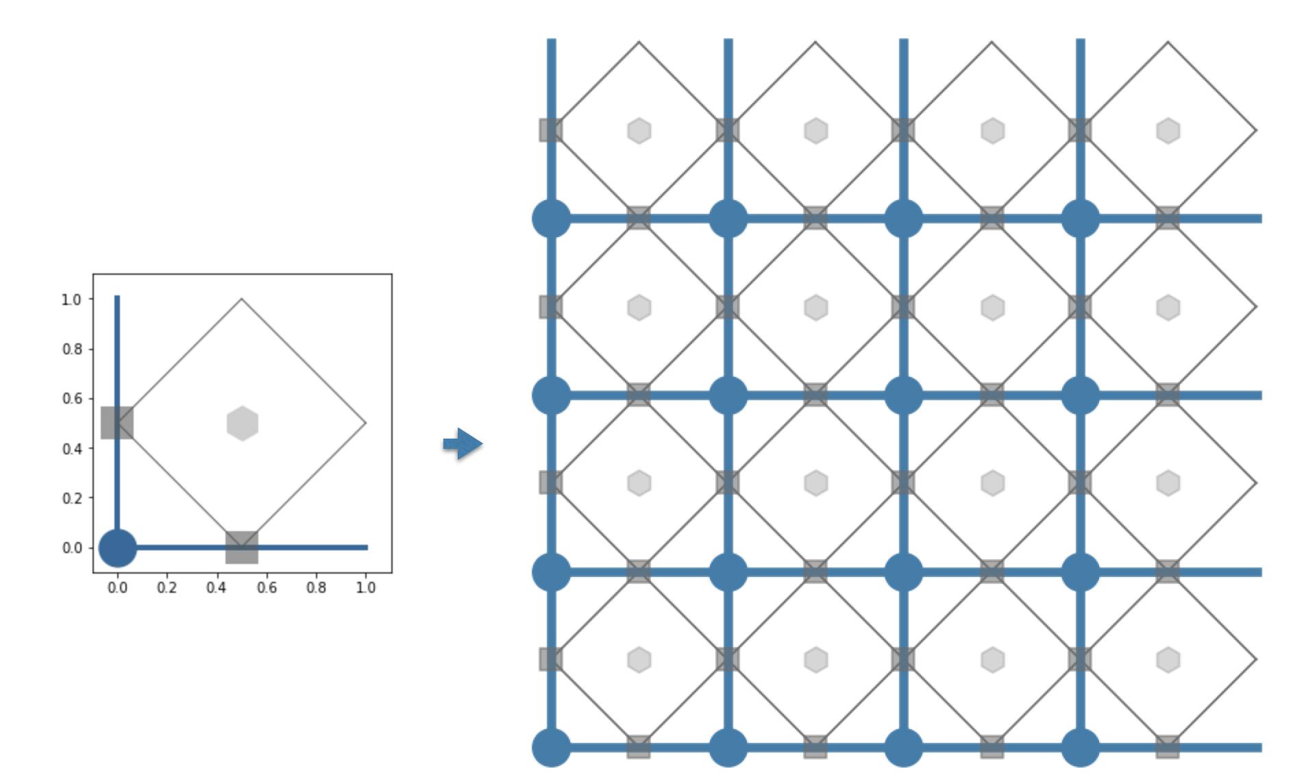
1. 绘制抽象的二维网格结构
catplot提供了丰富的接口用来定制所需要的任何二维网格并进行周期性扩展,如下图是一个通过当个重复单元扩展出来的抽象(100)晶面的二维网格结构:
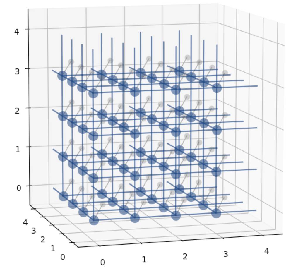
2. 绘制抽象的三维网格结构
同理只不过这次是在三维画布中进行绘制并进行重复单元的周期性扩展,扩展的效果如下图:
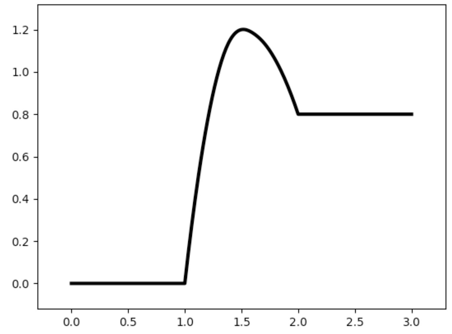
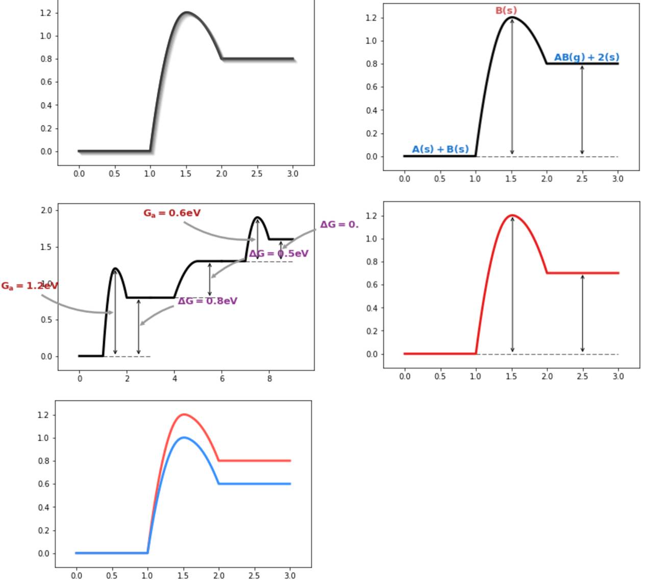
3. 通过插值算法实现绘制”顺滑”的energy profile
实现过程基本是通过对matplotlib提供的绘图组件和接口进一步封装成可以快速搭建上面三个类型图像的组件。
采用二次插值结合样条插值方法绘制 energy profile
energy profile可以理解成在势能面(Potential Energy Surface)上沿着某个特定的方向(反应坐标方向)上能量的变化,
下面我就上一个简单的例子来画一条顺滑的energy profile, 更多具体的例子我都已经jupyter notebook的形式放在的github上(https://github.com/PytLab/catplot/tree/master/examples)
# 从catplot中导入绘制所需的组件: 画布 和 线
from
catplot
.
ep_components
.
ep_canvas
import
EPCanvas
from
catplot
.
ep_components
.
ep_lines
import
ElementaryLine
# 创建一个用于绘制energy profile的画布
canvas
=
EPCanvas
()
# 创建一条能量曲线,提供的三个值分别是三个状态下的能量数值
line
=
ElementaryLine
([
0.0
,
1.2
,
0.8
])
# 将这条线添加到画布中
canvas
.
add_line
(
line
)
# 绘制
canvas
.
draw
()
canvas
.
figure
.
show
()
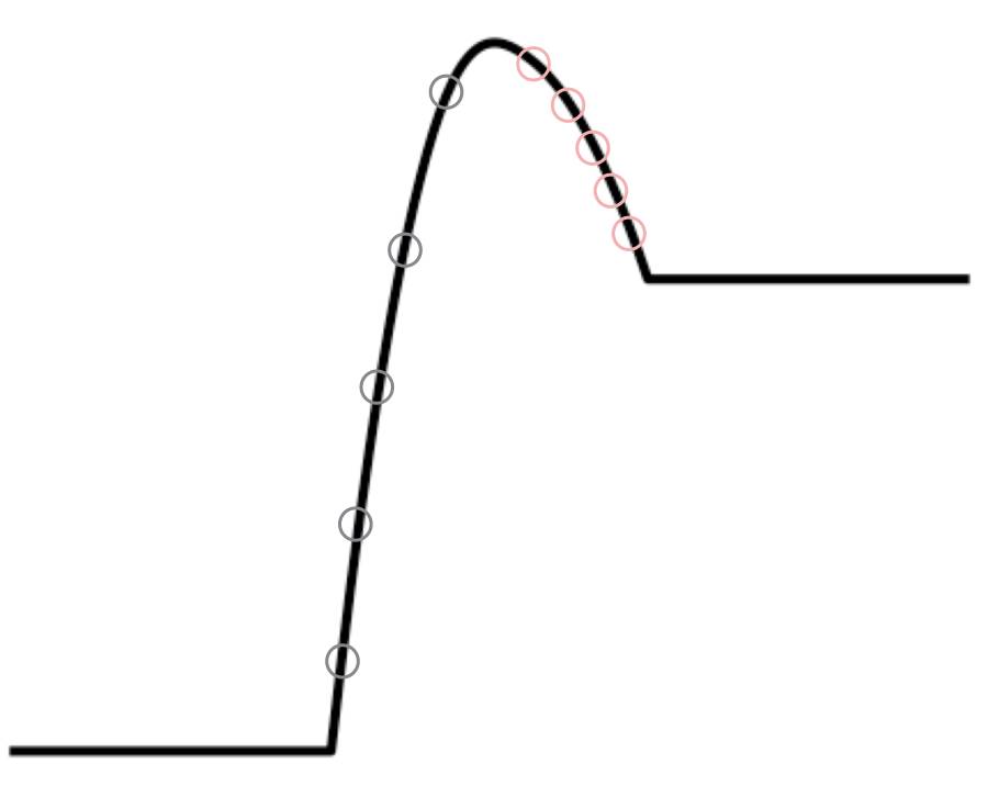
插值方法
为了能将能量最高点沿着横坐标任意位置移动,我先将顶点的两边用二次函数进行插值,获取两个不同的二次函数形式,然后根据二次函数的形式在左右两边插上5个点,为了能让分开插值的两部分看起来连续,在将上面的10个新插的点和之前的3个点进行一次spline插值即可。
# 顶点两侧进行二次插值的算法
def
quadratic_connect_interp
(
x1
,
y1
,
x2
,
y2
)
:
A
=
np
.
matrix
([[
x1
**
2
,
x1
,
1
],
[
x2
**
2
,
x2
,
1
],
[
2
*
x2
,
1
,
0
]])
b
=
np
.
matrix
([[
y1
],
[
y2
],
[
0
]])
x
=
A
.
I
*
b
x
.
shape
=
(
1
,
-
1
)
a
,
b
,
c
=
x
.
tolist
()[
0
]
poly_func
=
lambda
x
:
a
*
x
**
2
+
b
*
x
+
c
return
poly_func
与插值相关的方法参考:https://github.com/PytLab/catplot/blob/master/catplot/interpolate.py
丰富的接口
除了上面最简单的例子,catplot还提供了丰富的接口来定制和操作energy profile,比如拼接,合并,平移,添加阴影、改变颜色, 辅助线, 修改画布大小,导出插值数据等等。具体的例子参考: https://github.com/PytLab/catplot/tree/master/examples
绘制二维和三维抽象网格
晶格中的原子和键在catplot中被抽象成图中的node和edge,这样我们就可以通过创建图中的node和edge的方式搭建我们网格的重复单元,之后可以通过重复单元的扩展方法来将其扩展成nxn或者nxnxn的网格。
实现的基本方法就是通过matplotlib提供的Line2D, Arrow和scatter相关的接口来将相应node和edge的数据添加到maptlotlib的二维或者三维画布中然后进行绘制和显示。下面给分别给出两个绘制正交网格的绘制方法:
绘制5×5的二维网格
notebook版可以参见:https://github.com/PytLab/catplot/blob/master/examples/grid_2d_examples/expand_supercell.ipynb
创建nodes和edges
from
catplot
.
grid_components
.
nodes
import
Node2D
from
catplot
.
grid_components
.
edges
import
Edge2D
nodes
,
edges
=
[],
[]
# 创建重复单元中的nodes和edge
top
=
Node2D
([
0.0
,
0.0
],
size
=
800
,
color
=
"#2A6A9C"
)
t1
=
Node2D
([
0.0
,
1.0
])
t2
=
Node2D
([
1.0
,
0.0
])
nodes
.
append
(
top
)
# 链接这三个node的edges
e1
=
Edge2D
(
top
,
t1
,
width
=
4
)
e2
=
Edge2D
(
top
,
t2
,
width
=
4
)
edges
.
extend
([
e1
,
e2
])
# 中间的nodes
bridge1
=
Node2D
([
0.0
,
0.5
],
style
=
"s"
,
size
=
600
,
color
=
"#5A5A5A"
,
alpha
=
0.6
)
bridge2
=
Node2D
([
0.5
,
0.0
],
style
=
"s"
,
size
=
600
,
color
=
"#5A5A5A"
,
alpha
=
0.6
)
b1
=
bridge1
.
clone
([
0.5
,
0.5
])
b2
=
bridge2
.
clone
([
0.5
,
0.5
])
nodes
.
extend
([
bridge1
,
bridge2
])
# 连接他们的edges
e1
=
Edge2D
(
bridge1
,
b1
)
e2
=
Edge2D
(
bridge1
,
bridge2
)
e3
=
Edge2D
(
bridge2
,
b2
)
e4
=
Edge2D
(
b1
,
b2
)
edges
.
extend
([
e1
,
e2
,
e3
,
e4
])
# 正中间的node
h
=
Node2D
([
0.5
,
0.5
],
style
=
"h"
,
size
=
700
,
color
=
"#5A5A5A"
,
alpha
=
0.3
)
nodes
.
append
(
h
)
好了,现在我们就创建一个重复单元中的所需的所有元素,可以绘制一下看看效果了
from
catplot
.
grid_components
.
grid_canvas
import
Grid2DCanvas
from
catplot
.
grid_components
.
supercell
import
SuperCell2D
canvas
=
Grid2DCanvas
()


